They only display a chart? No values? What is the platform?
If that is just a plot, I am inclined to say all they do is to run Black Scholes, shorten the time (if you go 6m into the future, just make the expiry 6m shorter), and reprice with a few different spot values. I don't think there is anything fancy. If it's a bit more sophisticated, the vol would adjust, using the fact that tenor is now shorter and you move along the term structure. However, you ruled that out by writing it uses current (and optional vol). So you also do not move along the smile.
In Julia, you could do this in a few lines of code to get Black Scholes in a DataFrame:
using Plots, Distributions,DataFrames, PlotThemes
theme(:juno)

N(x) = cdf(Normal(0,1),x)

function BSM(S,K,t,rf,d,σ)
  d1 = ( log(S/K) + (rf - d + 1/2*σ^2)*t ) / (σ*sqrt(t))
  d2 = d1 - σ*sqrt(t)
  c  = exp(-d*t)S*N(d1) - exp(-rf*t)*K*N(d2)
  return c
end

S = 6:0.1:15 # spot range
t = 1        # start tenor (1 year)
shift = 6    # months shift
t_new = t - shift/12
df = DataFrame(Call = BSM.(S,10,t_new,0.0,0.0,0.2))
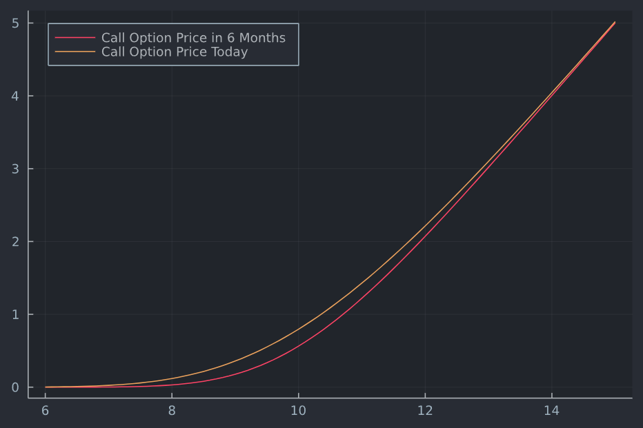
You can plot current value (assuming all else equal but spot changes) vs some day in the future (all that changes is the term to maturity; and spot).
plot(S,df.Call , label = "Call Option Price in 6 Months")
plot!(S,BSM.(S,10,t,0.0,0.0,0.2),
                label = "Call Option Price Today",
                legendposition = :topleft)

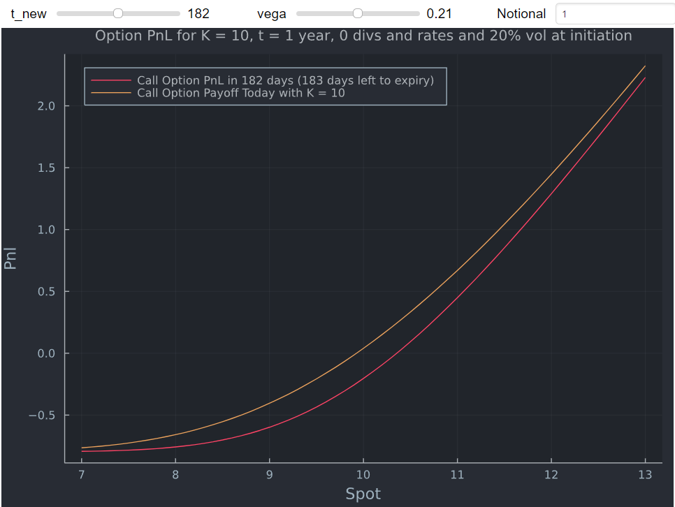
Adding a few lines computes the PnL (subtract initial cost), makes it dynamic (with slider for term and vol) and also allows you to play around with different notional values.
original_cost = BSM.(10,10,t,0.0,0.0,0.2)

function call(N, t_new, σ)
    payoff_call = N.*(BSM.(S,10,t-t_new/365.0,0.0,0.0,σ) .- original_cost)
end

function start_val(N, σ)
    payoff = N.*(BSM.(S,10,t,0.0,0.0,σ) .- original_cost)
end

S = 7:0.1:13
using Interact
call_gui = @manipulate for t_new = 1:1:364, σ = 0.01:0.01:0.41,
           Notional = spinbox(label="Notional"; value=1);

        plot(S,call(Notional, t_new, σ),
                label = "Call Option PnL in $t_new days ($(t*365-t_new) days left to expiry)",
                legendposition = :topleft,
                size = (800,500))

        plot!(S, start_val(Notional, σ),
                label = "Call Option Payoff Today with K = 10",
                xlabel = "Spot",
                ylabel = "Pnl",
                size = (700,500),
                title = "Option PnL for K = 10, t = 1 year, 0 divs and rates and 20% vol at initiation",
                titlefontsize=10)
end
@layout! call_gui vbox(hbox(:t_new, :σ, :Notional),observe(_))

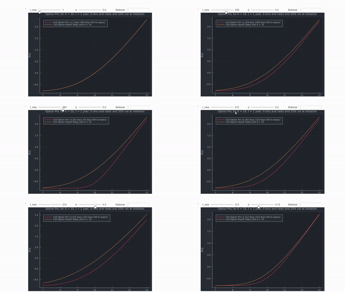
And changing a few params:

Now most equity markets are American, but in my example, the results would be identical for an American option anyways. In more general cases, you would need to implement this with a model that prices American options (PDE solver for example). You could also display the actual values in a DataFrame as opposed to just the chart.

