Return to Answer

The values are quick to replicate:

See the following screenshot from Bloomberg's OVML, where the 3rd screenshot has 25D as an input and solves for strike (the exact decimals are shown in white - when you hover over the value in the OVML screen).

The values are quick to replicate:

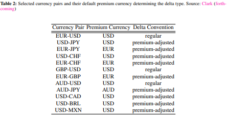
Since FX is all OTC, you can never be sure about the details unless you ask your broker. Generally though, in order to maintain liquidity there are a number of standardized conventions. Unfortunately, these conventions vary between currency pairs. Usually, vanilla EURUSD options are not premium adjusted.

If you have access to Bloomberg, you can check on OVDV - 92)Settings->Conventions. Wystup and Reiswich, 2009 also have an overview of the most commonly used conventions.

The values are quick to replicate:

• For CCY1CCY 2, you have Notional in CCY1 (20MM) and Premium in CCY2 (USD)
• You have a deferred (forward) premium, therefore I use two dates (see here for an explanation)
• all other inputs are given
• The model is just standard Garman Kohlhagen
• all inputs are provided in the question

In Julia, this looks as follows:

#load packages
using Distributions, Dates, DataFrames, PrettyTables
#define helper functions
ppf(x) = quantile(Normal(0.0, 1.0),x)
N(x) = cdf(Normal(0,1),x)

#define GK
function GK(F,K, days_to_expiry, days_to_delivery ,ccy1, ccy2,σ)
    d1 = ( log(F/K) +  0.5*σ^2*days_to_expiry/365 ) / (σ*sqrt(days_to_expiry/365))
    d2 = d1 - σ*sqrt(days_to_expiry/365)
    c  = exp(-ccy2*days_to_delivery/365)*(F*N(d1) - K*N(d2))
    δ_spot = exp(-ccy1*days_to_expiry/365) * N(d1)
    δ_fwd = N(d1)
  return c, δ_fwd, δ_spot
end

The inputs are all given, but the days to expiry and delivery are computed. I allow for hours to expiry but that is irrelevant here (the computed price is below the quoted, and delta would increase with increasing time).

# inputs 
s = 1.0615
pts = 60.1
fwd_scale = 10^4
f = s + pts / fwd_scale
println("Forward = $f")
k = 1.101
σ = 0.089
ccy1 = 0.0255008 #0.0255 # EUR
ccy2 = 0.0478 # USD

price_dt = Date(2023,3,16)
premium_dt = Date(2023,6,20)
expiry_dt = Date(2023,6,16)
delivery_dt = Date(2023,6,20)
hours =  0 #0.7115  allows to get more accurate pricing but more hours to expiry would be needed (increases delta)
days_to_expiry = (expiry_dt - price_dt).value + hours/24
days_to_delivery = (delivery_dt - premium_dt).value + hours/24
r1_cont = log(1+ccy1*days_to_expiry/360)/(days_to_expiry/365)
r2_cont = log(1+ccy2*days_to_expiry/360)/(days_to_expiry/365)

I am omitting PrettyTables formatting. Essentially, I compute strike for 25D according to Wystup and Reiswich, 2009 (omitting the call/put flag φ because we only care about calls here):

$$ K = fe^{-N^{-1}(e^{rf\tau} * \delta_{s})*\sigma* \sqrt{t} + \frac{1}{2}*\sigma^{2}*\tau }$$ or for forward delta: $$ K = fe^{-N^{-1}(\delta_{f})*\sigma* \sqrt{t} + \frac{1}{2}*\sigma^{2}*\tau }$$

δ = 0.25
# compute strike from delta 
k_25D    = f*exp((1/2)*σ^2*days_to_expiry/365 - ppf(δ*exp(r1_cont *days_to_expiry/365))*σ*sqrt(days_to_expiry/365))
# get option value for computed strike and quoted strike 
opt  = [GK(f, strike, days_to_expiry, days_to_delivery, r1_cont, r2_cont, σ) for strike in (k, k_25D)]
# get spot premium 
premium_dt_spot = Date(2023,3,20)
days_to_delivery_spot = (delivery_dt - premium_dt_spot).value + hours/24
opt2 = [GK(f, strike, days_to_expiry, days_to_delivery_spot, r1_cont, r2_cont, σ) for strike in (k, k_25D)];
Notional = 20_000_000
df = DataFrame("Strike" => [k, k_25D], 
                "Fwd Premium USD" => [opt[1][1]*Notional, opt[2][1]*Notional ], 
                "Spot Premium USD" => [opt2[1][1]*Notional ,opt2[2][1]*Notional ], 
                "Fwd Delta" => [opt[1][2]*100 , opt[2][2]*100 ], "Spot Delta" => [opt[1][3]*100, opt[2][3]*100] )

The output matches Bloomberg exactly:

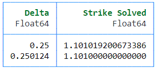
Using the computed spot delta of 25.0124 returns the strike (1.101):

DataFrame("Delta" => [δ, opt[1][3]], "Strike Solved" => [k_25D, f*exp((1/2)*σ^2*days_to_expiry/365 - ppf(opt[1][3]*exp(r1_cont *days_to_expiry/365))*σ*sqrt(days_to_expiry/365))])

P.S. If it were premium included, you would not be able to use a closed form solution and would need to solve for strike numerically - for example, using Brent's root-finding method as suggested by Wystup and Reiswich.

However, since you directly want the Bloomberg values, you can simply use the API for a convenient solution that matches OVDV by design.

It seems your end goal is to get a vol associated with some strike and tenor. In Bloomberg, you can actually let the API do that "trick" for you, including all conventions (premium included / excluded; spot / fwd delta...) and settings you have on the terminal.

For the strike override to work, you 1st have to set the delta override to 0 because that delta is used by default and that is the way to exclude it in the API.

=BDP("EURUSD Curncy","SP_VOL_SURF_BID","VOL_SURF_EXPIRY_OVR","20221030","VOL_SURF_CALLPUT_OVR","C","REFERENCE_DATE","20220324","VOL_SURF_DELTA_OVR","0","VOL_SURF_STRIKE_OVR=1.25”)

This gives you for the date 2022-03-24 the EURUSD call IVOL for expiry on 2022-10-30 and a strike of 1.25.

You can also use tenors directly like so:

=BDP("GBPUSD Curncy","SP_VOL_SURF_MID","VOL_SURF_MTY_OVR=1D","VOL_SURF_CALLPUT_OVR=P","VOL_SURF_STRIKE_OVR=1.1","VOL_SURF_DELTA_OVR=0")

It seems your end goal is to get a vol associated with some strike and tenor. In Bloomberg, you can actually let the API do that "trick" for you, including all conventions (premium included / excluded; spot / fwd delta...) and settings you have on the terminal.

For the strike override to work, you 1st have to set the delta override to 0 because that delta is used by default and that is the way to exclude it in the API.

=BDP("EURUSD Curncy","SP_VOL_SURF_BID","VOL_SURF_EXPIRY_OVR","20221030","VOL_SURF_CALLPUT_OVR","C","REFERENCE_DATE","20220324","VOL_SURF_DELTA_OVR","0","VOL_SURF_STRIKE_OVR=1.25”)

This gives you for the date 2022-03-24 the EURUSD call IVOL for expiry on 2022-10-30 and a strike of 1.25.

You can also use tenors directly like so:

=BDP("GBPUSD Curncy","SP_VOL_SURF_MID","VOL_SURF_MTY_OVR=1D","VOL_SURF_CALLPUT_OVR=P","VOL_SURF_STRIKE_OVR=1.1","VOL_SURF_DELTA_OVR=0")

If you really want to do it yourself, you can look at this answer which shows in formula and code how Bloomberg solves for strike from delta. Bear in mind, this doesn't work if premium adjusted while the excel formula above just does everything correctly for you and pulls the correct IV for any strike and tenor you wish.