Empirical analysis of realized measures

The paper Does anything beat 5-minute RV? A comparison of realized measures across multiple asset classes [LPS2015] does a very good job of defining a scalable comparison framework for realized measures and models. The theory behind many of the methods is developed in different papers cited in the study. I will briefly highlight the applicational framework of the comparison analysis which can be coded in R.

I have provided some very simple R code which can be extended to multiple realized measures and comparison methods. The purpose is to give you a framework and not a complete solution. The R code can be found in an appendix.

The Setup:

The general framework from the paper can be outlined as follows:

1. Determine the cleaning procedure, sampling scheme and the frequency of your data.

2. Determine the realized measures under investigation.

3. Find the proxy and perform Data-based ranking method.

4. Preliminary analysis of the assets.

5. Comparison analysis using pair-wise and multiple comparison methods.

6. Linking volatility measures to models: Does the adequate performance of realized measure imply better out-of-sample forecasts for the models?

You can extend (4), (5), and (6) however you want. [LPS2015] is very exhaustive when doing the analysis in (4), (5) and (6). It is not necessary to pick out this many comparison methods in (5). If you want to work with multiple realized measure then choose one multiple comparison method and move on. In this case, the Model Confidence Set is very popular and is already implemented in R.

Data & preliminary cleaning:

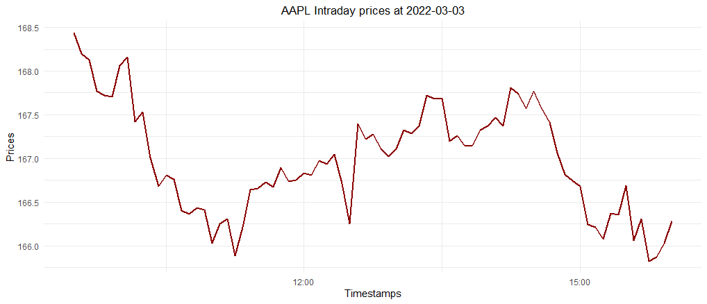
I have omitted (1), (2) and focused more on the data-based ranking method of (Patton, 2011). Moreover, I have downloaded free 5-minute stock prices for AAPL from the website AlphaVantage.co. Intraday data is freely available (in a limited amount) for anyone who has an API key (you can get one for free). After an ad-hoc preliminary cleaning the intraday close-prices at a random day, looks like this:

The two realized measures I have under investigation in my R code, is the Realized Variance (RV) and the Bipower Realized variance:

$$ RV_t = \sum_{i=1}^n r_{i,t}^2 \qquad \quad BPRV_t = \sum_{i=1}^{n-1} |r_{i+1,t}| \cdot |r_{i,t}|, $$ for $n$ being the amount of intraday data at each day $t$.

3. Find the proxy and perform Data-based ranking method

Patton's data-based ranking method estimates the relative accuracy between two realized measures $\Sigma_{it}, \: \Sigma_{jt}$, using a loss function $L(\cdot)$ based on a proxy of the latent volatility process $\theta$:

\begin{equation} \mathbb{E}\left[\Delta L(\theta_t, \Sigma_t)\right] = \mathbb{E}\left[L(\theta_t, \Sigma_{it}) - L(\theta_t, \Sigma_{jt})\right]. \end{equation}

When $T \rightarrow \infty$ the above equation can be consistently estimated via, \begin{equation}\label{meanloss} d_{ij}=\frac{1}{T} \sum_{t=1}^{T} \Delta \hat{L}_{ij,t} \overset{\mathbb{P}}{\longrightarrow} \mathbb{E}\left[\Delta L_{ij,t}\right], \end{equation} where $\Delta \hat{L}_{ij,t} = L(\theta_t, \Sigma_{it}) - L(\theta_t, \Sigma_{jt})$ and $\Delta L_{ij,t}$ being the loss difference.

Things to consider:

We need to consider the choice of loss-function and volatility proxy. Here are some highlights from the original paper that makes this relatively straight forward:

1. A proper Loss function: (Patton, 2011) argues that a "robust" loss function together with a conditional unbiased volatility proxy (of the latent volatility process) in the rankings of volatility forecasts, are asymptotically equivalent to rankings using the true latent volatility variable. He further argues that the robust loss function will be invariant to the noise in the user-defined proxy. Two robust loss functions are the QLIKE and the MSE: $$ L^{\text{QLIKE}}(\theta, \Sigma) = \frac{\theta}{\Sigma} - \ln\left(\frac{\theta}{\Sigma}\right) - 1 \qquad L^{\text{MSE}}(\theta, \Sigma) = (\theta - \Sigma)^2 $$ where $\theta$ denote the proxy of the true latent volatility process and $\Sigma$ is your realized estimator under investigation.

2. Determine a proxy for the true latent volatility process: In [LPS2015] they use the daily sampled RV as proxy with a lead-lag proposition. This proxy is also the choice in (Patton, 2011). The lead-lag proposition determines how good todays realized volatility estimate is as a forecast for tomorrow volatility. Not only that, but it also breaks the dependence between the proxy and the realized measures. In conclusion, this implies that they calculate the loss of the estimated forecast of tomorrows realized variance $\mathbb{E}\left[RV^{\text{5 min}}_{t+1} \vert \mathcal{F}_t\right] = RV^{\text{5 min}}_t$ with the ex-post (estimated on day $t+1$) daily realized variance, $RV^{\text{daily}}_{t+1}$.

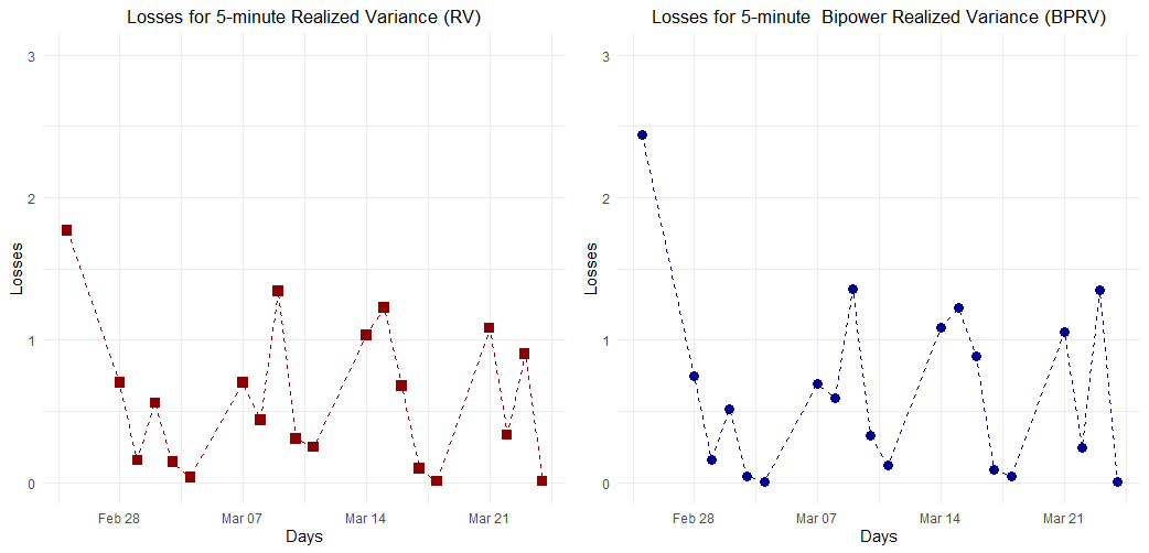
Looking at the R code you will notice that I have used the Realized Variance sampled daily (open-to-close) as my proxy and the corresponding QLIKE losses function. A graph is presented below, that shows the losses across days for two realized measures, Realized variance (RV) and Bipower Realized Variance (BPRV) on a 5-minute sampling frequency of AAPL:

4 & 5. Ranking measures and comparison analysis

In LPS2015 they do a small study on the assets themselves which includes summary statistics and an ad-hoc liquidity analysis by looking at the trade- and quote-duration in seconds. Other than that, they start their main analysis by employing different pair-wise and multiple comparison methods. All of the comparison methods are described in my answer here and my answer also contains a link to Python implementation of these measures. With regards to R then the Diebold-Mariano test is implemented in the forecast package here and there exists a package for the Model Confidence Set (link).

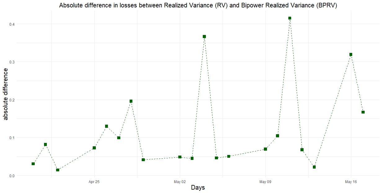
If we utilize a Diebold-Mariano test (with pre-defined parameters given in the function) on our simple example, we get a $p$-value of $p=0.1578$ and therefore we fail to reject the null hypothesis of equal predictive power. Obviously, the results might look different for longer horizons and for different financial products. Doing the same pair-wise comparison for 20 different stocks (omitted from appendix code) the proportion of rejections is only 10%, implying that 2 out of the 20 stocks we failed to reject the null. In these two cases BPRV outperformed RV in terms of lower average loss, $d_{ij}$.

6. Out-of-sample investigation

In the last bit of their empirical investigation they utilize a Heterogeneous Autoregressive (HAR) model, that linearly combines different volatility components formed from the expected realized estimates over different horizons. For clarity, let us define the volatility components of the HAR model as: \begin{equation} RV_{t-1}^{(day)} = RV_{t-1}^{(n)}, \qquad RV_{t-1}^{(week)} = \frac{1}{5}\sum_{k=1}^{5}RV_{t-k}^{(n)}, \qquad RV_{t-1}^{(month)} = \frac{1}{22}\sum_{k=1}^{22}RV_{t-k}^{(n)}, \end{equation} assuming 22 days in a month, and $n$ being the amount of intraday data. Then, the HAR model can be described as, \begin{equation} RV_t = \phi_0 + \phi_1 RV_{t-1} +\phi_2 RV_{t-1}^{(week)} + \phi_3 RV_{t-1}^{(month)} + u_t, \end{equation} where you can replace $RV_t$ with any realized measure giving you alternative formulations of the HAR model. As an example I have provided a description of the SHAR model that disentangles the Realized Variance (RV) into a positive and negative semi-variation. Also, Inserting the Bipower Realized Variance gives you the Continuous HAR (CHAR) model, since Bipower variation is a jump-robust measure, and thus only includes measures of continuous variation.

In their empirical study they estimate the model for different forecast horizons from $h=1,\ldots,50$, compares the forecasts with the ex-post realized values and outputs the proportion of times the 5-minute realized variance is included in the best set of measure across different asset types. This is another extensive analysis and instead you could focus on a 1-step ahead forecast analysis with your own choice of comparison method. Be aware that the adequate realized measure chosen in a preliminary study, might not outperform in the out-of-sample investigation. I haven't coded this part since I lacked data and time.

Appendix

######################### TOY EXAMPLE ###########################

####### packages
library(xts)
library(forecast)
library(highfrequency)
library(alphavantager)
library(ggplot2)
av_api_key("YOUR API KEY HERE")



############ GET DATA AND DO DATA CLEANING:

# Get time-series data (Intraday)
AAPL <- as.data.frame(av_get(symbol = "AAPL", av_fun = "TIME_SERIES_INTRADAY", 
  outputsize = "full", interval = '5min'))
rownames(AAPL) <- AAPL$timestamp

# Preliminary data-cleaning
AAPL_close <- xts(AAPL$close, order.by = AAPL$timestamp)

#split into days (list object)
AAPL_close <- split(AAPL_close, as.Date(index(AAPL_close)))

#ad-hoc deleting pre- and after-market hours
AAPL_close <- lapply(AAPL_close, function(x){ 

    premarketdel <- grep("09:30:00", 
      format(index(x), format = "%H:%M:%S"))

    aftermarketdel <- grep("16:05:00", 
      format(index(x), format = "%H:%M:%S"))

    x[-c(1:(premarketdel - 1), aftermarketdel:length(x))]
    }
  )

# intraday returns
AAPL_ret <- lapply(AAPL_close, function(x) diff(log(x))[-1])


############# REALIZED MEASURES 

# These are just examples.

# Realized variance 
RV <- sapply(AAPL_ret, function(x) rCov(x, makeReturns = FALSE))

# Bipower realized variance
BPRV <- sapply(AAPL_ret, function(x) rBPCov(x, makeReturns = FALSE))


############# Pattons databased ranking method. 

#proxy is open to close RV:
RVDAILY <- sapply(AAPL_close, function(x) (log(as.numeric(x[length(x)])) - log(as.numeric(x[1])))^2)

#Loss function, QLIKE:
Qlike <- function(proxy, realized){

  loss <- proxy / realized - log( proxy / realized ) - 1

  return(loss)

}

#Lag the RV
LagRVDAILY <- dplyr::lag(RVDAILY, 1)[-1]

### Calculate the losses using the lead-lag proposition
LossRV <- Qlike(LagRVDAILY, RV[-length(RV)])

LossBPRV <- Qlike(LagRVDAILY, BPRV[-length(BPRV)])


# Now see that d_{ij} = mean(LossRV - LossBPRV). However, this was not needed in my simple analysis.


############# VERY SIMPLE COMPARISON METHOD 

dm.test(LossRV, LossBPRV)


############# PLOTS. 

# PLOT 1
ggplot() + geom_line(aes(index(AAPL_close[[6]]), AAPL_close[[6]]), col = "darkred", lwd = 1)+ 
xlab("Timestamps") + ylab("Prices") + theme_minimal() + 
ggtitle("AAPL Intraday prices at 2022-03-03") + 
 theme(legend.position = "none", 
  plot.title = element_text(hjust = 0.5) 
  ) 

# PLOT 2
p1 <- ggplot() +  geom_point(aes(as.Date(names(AAPL_close[-1])), LossRV), shape=15, 
  fill = "darkred", color="darkred", size = 3) + 
geom_line(aes(as.Date(names(AAPL_close[-1])), LossRV),col = "darkred", linetype = "dashed") +
ggtitle("Losses for 5-minute Realized Variance (RV)") + ylab("Losses") + xlab("Days") + 
ylim(c(0,3)) +  theme_minimal() + 
 theme(legend.position = "none", 
  plot.title = element_text(hjust = 0.5) 
  ) 


p2 <- ggplot() + geom_point(aes(as.Date(names(AAPL_close[-1])), LossBPRV), shape=16, 
  fill = "darkblue", color="darkblue", size = 3) +
geom_line(aes(as.Date(names(AAPL_close[-1])), LossBPRV),col = "darkblue", linetype = "dashed") + 
ylab("Losses") + xlab("Days") + ggtitle("Losses for 5-minute  Bipower Realized Variance (BPRV)") +
ylim(c(0,3)) +  theme_minimal() + 
 theme(legend.position = "none", 
  plot.title = element_text(hjust = 0.5) 
  ) 


library(gridExtra)
grid.arrange(p1, p2, ncol = 2)