Non-convergence in Monte Carlo

Question

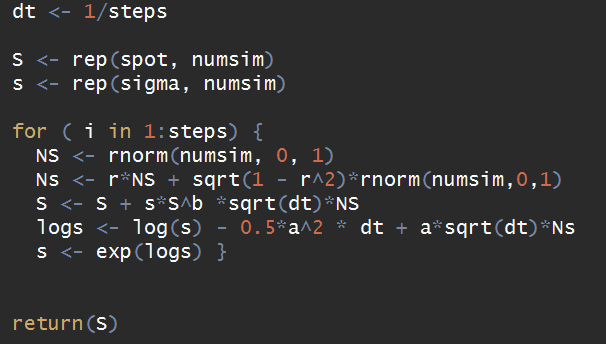
Trying to implement some monte carlo simulation for the first time. For the sabr model (http://www.javaquant.net/papers/managing_smile_risk.pdf), would this work?

Here, a = volatility of volatility, and s = volatility, and r = correlation of wiener processes.

If its ok, then why does it not produce the same results as the SABR formula does?

What I do is that I simulate S_T, then I compute max(S_T - K,0) for every simulation, and then calculate average. For some parameter choices, I get the same as SABR, but for others, I get the wrong number, even if I ramp up the sample and time steps.

So it my code wrong? Is the SABR formula wrong? Which technique produces correct results?

Answer 1

I can see two potential issues here:

Discretization Scheme

First, you should consider different simulation schemes. In the special case of constant volatility ($\alpha = 0$), the SABR model reduces to the CEV model. The basic Euler scheme that you employ for the spot process has been show to exhibit a significant bias for this process. See Lord (2014) and Chen et al. (2011) for an in depth-discussion and comparison of more advanced simulation schemes.

"SABR Formula"

I suppose that you refer to the second order expansion in Equation (2.17) of Hagan et. al (2002) as the "SABR Formula". As the name suggests this is only an approximation for the implied volatility. Furthermore, it is known to not be free of arbitrage (e.g. for very low strikes).

References

Lord, Roger (2014) "Fifty Shades of SABR Simulation," 10th Fixed Income Conference, Barcelona, available here

Chen, Bin, Cornelis W. Oosterlee and Hans van der Weide (2011) "Efficient Unbiased Simulation Scheme for the SABR Stochastic Volatility Model," Working Paper, TU Delft, available here

Hagan, Patrick S, Deep Kumar, Andrew S. Lesniewski and Diana E. Woodward (2002) "Managing Smile Risk," Wilmott Magazine

Answer 2

Although for a special case of normal SABR ($\beta=0$), there is an exact closed-form MC simulation scheme which does not require discretization in time. See my paper, Hyperbolic normal stochastic volatility model (arXiv | SSRN | DOI)

Answer 3

Perhaps you can give a few cases where your code does not reproduce the SABR formula.

Fix beta=1 and start with a=0. This should reduce to the Black-Scholes model. The code should match the BS formula. Then increase the vol-of-vol a, first with zero correlation and then changing it to some non-positive value, e.g. -0.7.

Answer 4

The SABR formula is wrong. There is a set of papers that begins with a solution for the distribution that must be present for all asset classes and a paper to verify the distribution present. It provides a mathematical reason for Mandelbrot's 1963 paper, On the Variation of Certain Speculative Prices.

The difficulty with a Bayesian method is that if your model is wrong, it should get flat and then it will take much much longer to converge. The distribution of returns for a stock that is a going concern is $$\left[\frac{\pi}{2}+\tan^{-1}\left(\frac{\mu}{\gamma}\right)\right]^{-1}\frac{\gamma}{\gamma^2+(r-\mu)^2}$$ in a world with no liquidity concerns.

This would be multiplied either by an adjustment for the bid-ask spread or for the probability that a trade would happen given the budget constraint of the counter-party was met.

The big issue here is that $\gamma$ does not satisfy the definition of variance. If you try to solve the integral for the first or second moment, it diverges. This is the source of the heavy tails. The logic is that a return is a future value divided by a present value minus one. Ignoring the minus one component since it is just a translation, this implies that a return is a ratio distribution. Under suitable circumstances, the distribution above would be that ratio distribution.

If you were to do it as a multiplication instead, that is $p_{t+1}=\beta{p_t}+\epsilon_{t+1}$ then by a proof by White in 1958 the residuals diverge hopelessly and there is no non-Bayesian solution as a result. The Bayesian solution is $$\frac{1}{\pi}\frac{\gamma}{\gamma^2+(r-\mu)^2}.$$ This also has no moments.

If you are associated with a statistician, you can verify this. You can also verify it at http://mathworld.wolfram.com/RatioDistribution.html and at http://mathworld.wolfram.com/CauchyDistribution.html