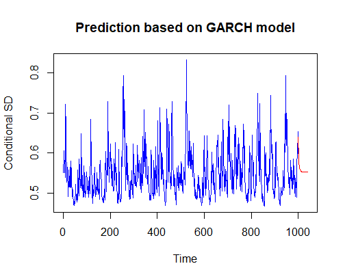
Here's a reproducible example using the package fGarch, I hope you can adapt it to your situation:

library("fGarch")

# Create specification for GARCH(1, 1)
spec <- garchSpec(model = list(omega = 0.05, alpha =  0.1, beta = 0.75), cond.dist = "norm")

# Simulate the model with n = 1000
sim <- garchSim(spec, n = 1000)

# Fit a GARCH (1, 1)
fit <- garchFit(formula = ~ garch(1, 1), data = sim, include.mean = F)

# Predict 40 steps ahead
pred <- predict(fit, n.ahead = 40)

# Concatenate the fitted model with the prediction, transform to time series
dat <- as.ts(c(sqrt([email protected]), pred = pred$standardDeviation))

# Create the plot
plot(window(dat, start = start(dat), end = 1000), col = "blue",
     xlim = range(time(dat)), ylim = range(dat),
     ylab = "Conditional SD", main = "Prediction based on GARCH model")

par(new=TRUE)

plot(window(dat, start = 1000), col = "red", axes = F, xlab = "", ylab = "", xlim = range(time(dat)), ylim = range(dat))
A thank you to the writer of the answer in this thread, I used it to get the graphics right.
Also note that you can create a plot of the predicted series, rather than the predicted conditional standard deviation, by using the plot = T argument in the call to predict.

