We can demonstrate this via a pricing experiment using QuantLib-Python.
I've defined several utility functions in the code block at the bottom of the answer that you will need to replicate the work.
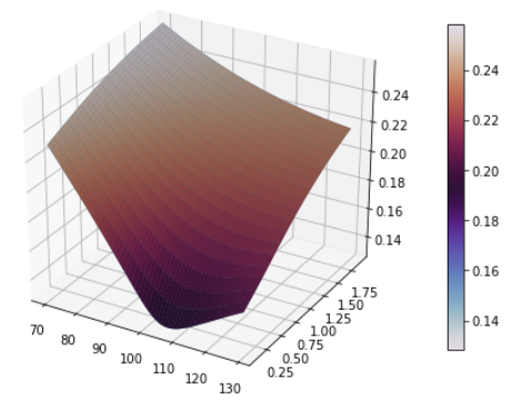
First, let's create a Heston process, and calibrate a local vol model to match it. Up to numerical issues, these should both price vanillas the same.
v0, kappa, theta, rho, sigma = 0.015, 1.5, 0.08, -0.4, 0.4

dates, strikes, vols, feller = create_vol_surface_mesh_from_heston_params(today, calendar, spot, v0, kappa, theta, rho, sigma, flat_ts, dividend_ts)

local_vol_surface = ql.BlackVarianceSurface(today, calendar, dates, strikes, vols, day_count)

# Plot the vol surface ...
plot_vol_surface(local_vol_surface, plot_years=np.arange(0.1, 2, 0.1))

Here, I've chosen the heston params to give a quite rapidly increasing vol, moderate downward skew, and to keep us safe from the feller condition.
Now the most elegant way to proceed would be to use inbuilt pricers in ql and price instruments of type ql.ForwardVanillaOption, but unfortunately the only forward option pricing engine currently exposed in python is ql.ForwardEuropeanEngine whihc will price under local vol but not under the heston model, so instead I proceed using monte carlo and pricing options explicitely (it's a bit rough but demonstrates the point).
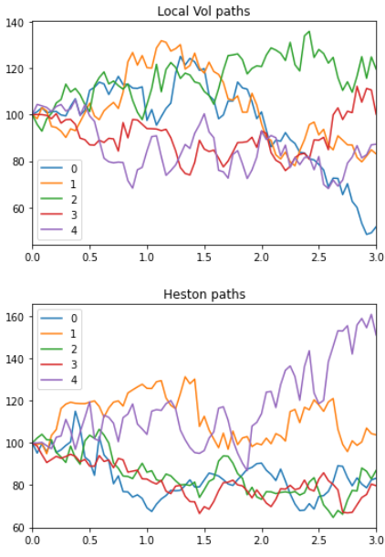
Next step, I generate many MC paths from the processes I just defined
local_vol = ql.BlackVolTermStructureHandle(local_vol_surface)

bs_process = ql.BlackScholesMertonProcess(ql.QuoteHandle(ql.SimpleQuote(spot)), dividend_ts, flat_ts, local_vol)
heston_process = ql.HestonProcess(flat_ts, dividend_ts, ql.QuoteHandle(ql.SimpleQuote(spot)), v0, kappa, theta, sigma, rho)

bs_paths = generate_multi_paths_df(bs_process, num_paths=100000, timestep=72, length=3)[0]
heston_paths, heston_vols = generate_multi_paths_df(heston_process, num_paths=100000, timestep=72, length=3)

bs_paths.head().transpose().plot()

plt.pause(0.05)

heston_paths.head().transpose().plot()

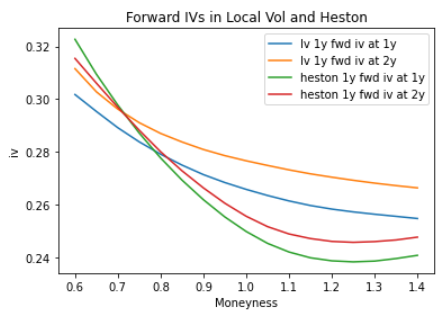
Now that we have paths, we want to price forward starting options along each one. Below, I price options starting at 1Y and expiring at 2Y, and options starting at 2Y and expiring at 3Y, at varying moneynesses (the strike is only determined at inception, by spot*moneyness). Since my rates are 0 everywhere, the price of these options is just (S(2) - moneyness * S(1)).clip(0).mean() or similar.
We also need to back out 'implied vols' from these prices. Since the strike isn't determined in advance it's not totally clear that using the regular BS formula is right, but I've done it anyway (using moneyness * spot as the strike), below.
moneynesses = np.linspace(0.6, 1.4, 17)
prices = []

for moneyness in moneynesses:
    lv_price_1y = (bs_paths[2.0] - moneyness * bs_paths[1.0]).clip(0).mean()
    lv_price_2y = (bs_paths[3.0] - moneyness * bs_paths[2.0]).clip(0).mean()

    heston_price_1y = (heston_paths[2.0] - moneyness * heston_paths[1.0]).clip(0).mean()
    heston_price_2y = (heston_paths[3.0] - moneyness * heston_paths[2.0]).clip(0).mean()

    prices.append({'moneyness': moneyness, 'lv_price_1y': lv_price_1y, 'lv_price_2y': lv_price_2y, 'heston_price_1y': heston_price_1y, 'heston_price_2y': heston_price_2y})

price_df = pd.DataFrame(prices)

price_df['lv_iv_1y'] = price_df.apply(lambda x: bs_implied_vol(x['lv_price_1y'], 1.0, 100, 100 * x['moneyness'], 1.0), axis=1)
price_df['lv_iv_2y'] = price_df.apply(lambda x: bs_implied_vol(x['lv_price_2y'], 1.0, 100, 100 * x['moneyness'], 1.0), axis=1)
price_df['heston_iv_1y'] = price_df.apply(lambda x: bs_implied_vol(x['heston_price_1y'], 1.0, 100, 100 * x['moneyness'], 1.0), axis=1)
price_df['heston_iv_2y'] = price_df.apply(lambda x: bs_implied_vol(x['heston_price_2y'], 1.0, 100, 100 * x['moneyness'], 1.0), axis=1)

plt.plot(moneynesses, price_df['lv_iv_1y'], label='lv 1y fwd iv at 1y')
plt.plot(moneynesses, price_df['lv_iv_2y'], label='lv 1y fwd iv at 2y')
plt.plot(moneynesses, price_df['heston_iv_1y'], label='heston 1y fwd iv at 1y')
plt.plot(moneynesses, price_df['heston_iv_2y'], label='heston 1y fwd iv at 2y')

plt.title("Forward IVs in Local Vol and Heston")
plt.legend()

As you can see, the forward vols coming from lv are much flatter and less smiley than the heston process prices, which is exactly the effect we were looking for.
Utility functions and QuantLib boilerplate code:
import warnings
warnings.filterwarnings('ignore')

import QuantLib as ql
import numpy as np
import pandas as pd

from scipy import optimize, stats
from matplotlib import pyplot as plt
import matplotlib.cm as cm
from mpl_toolkits.mplot3d import Axes3D

def plot_vol_surface(vol_surface, plot_years=np.arange(0.1, 3, 0.1), plot_strikes=np.arange(70, 130, 1), funct='blackVol'):
    if type(vol_surface) != list:
        surfaces = [vol_surface]
    else:
        surfaces = vol_surface

    fig = plt.figure(figsize=(8,6))
    ax = fig.gca(projection='3d')
    X, Y = np.meshgrid(plot_strikes, plot_years)

    for surface in surfaces:
        method_to_call = getattr(surface, funct)

        Z = np.array([method_to_call(float(y), float(x))
                      for xr, yr in zip(X, Y)
                          for x, y in zip(xr,yr) ]
                     ).reshape(len(X), len(X[0]))

        surf = ax.plot_surface(X,Y,Z, rstride=1, cstride=1, linewidth=0.1)

    N = Z / Z.max()  # normalize 0 -> 1 for the colormap
    surf = ax.plot_surface(X, Y, Z, rstride=1, cstride=1, linewidth=0.1, facecolors=cm.twilight(N))

    m = cm.ScalarMappable(cmap=cm.twilight)
    m.set_array(Z)
    plt.colorbar(m, shrink=0.8, aspect=20)
    ax.view_init(30, 300)

def generate_multi_paths_df(process, num_paths=1000, timestep=24, length=2):
    """Generates multiple paths from an n-factor process, each factor is returned in a seperate df"""
    times = ql.TimeGrid(length, timestep)
    dimension = process.factors()

    rng = ql.GaussianRandomSequenceGenerator(ql.UniformRandomSequenceGenerator(dimension * timestep, ql.UniformRandomGenerator()))
    seq = ql.GaussianMultiPathGenerator(process, list(times), rng, False)

    paths = [[] for i in range(dimension)]

    for i in range(num_paths):
        sample_path = seq.next()
        values = sample_path.value()
        spot = values[0]

        for j in range(dimension):
            paths[j].append([x for x in values[j]])

    df_paths = [pd.DataFrame(path, columns=[spot.time(x) for x in range(len(spot))]) for path in paths]

    return df_paths

def create_vol_surface_mesh_from_heston_params(today, calendar, spot, v0, kappa, theta, rho, sigma,
                                               rates_curve_handle, dividend_curve_handle,
                                               strikes = np.linspace(40, 200, 161), tenors = np.linspace(0.1, 3, 60)):
    quote = ql.QuoteHandle(ql.SimpleQuote(spot))

    heston_process = ql.HestonProcess(rates_curve_handle, dividend_curve_handle, quote, v0, kappa, theta, sigma, rho)
    heston_model = ql.HestonModel(heston_process)
    heston_handle = ql.HestonModelHandle(heston_model)
    heston_vol_surface = ql.HestonBlackVolSurface(heston_handle)

    data = []
    for strike in strikes:
        data.append([heston_vol_surface.blackVol(tenor, strike) for tenor in tenors])

    expiration_dates = [calendar.advance(today, ql.Period(int(365*t), ql.Days)) for t in tenors]
    implied_vols = ql.Matrix(data)
    feller = 2 * kappa * theta - sigma ** 2

    return expiration_dates, strikes, implied_vols, feller

def d_plus_minus(forward, strike, tte, vol):
    denominator = vol * np.sqrt(tte)
    inner_term = np.log(forward / strike) + 0.5 * vol * vol * tte
    d_plus = inner_term / denominator
    d_minus = d_plus - denominator

    return d_plus, d_minus

def call_option_price(vol, dcf, forward, strike, tte):
    d_plus, d_minus = d_plus_minus(forward, strike, tte, vol)
    return dcf * (forward * stats.norm.cdf(d_plus) - strike * stats.norm.cdf(d_minus))

def vol_solver_helper(x, price, dcf, forward, strike, tte):
    return call_option_price(x, dcf, forward, strike, tte) - price

def bs_implied_vol(price, dcf, forward, strike, tte):
    return optimize.brentq(vol_solver_helper, 0.0001, 2.0, args=(price, dcf, forward, strike, tte))

# World State for Vanilla Pricing
spot = 100
vol = 0.1
rate = 0.0
dividend = 0.0

today = ql.Date(1, 9, 2020)

day_count = ql.Actual365Fixed()
calendar = ql.NullCalendar()

# Set up the vol and risk-free curves
volatility = ql.BlackConstantVol(today, calendar, vol, day_count)
riskFreeCurve = ql.FlatForward(today, rate, day_count)
dividendCurve = ql.FlatForward(today, rate, day_count)

flat_ts = ql.YieldTermStructureHandle(riskFreeCurve)
dividend_ts = ql.YieldTermStructureHandle(dividendCurve)
flat_vol = ql.BlackVolTermStructureHandle(volatility)

