0
$\begingroup$

I have some technical questions about what are the best settings in Bloomberg to calculate the interest rate risk of a swap.

When Bloomberg calculates the DV01, it simply bumps the par swap curve by +/-10bps, then calculates the difference in NPVs, and divides it by 20. When Bloomberg does this, it does not touch the discount curve, only the par swap curve is being shifted which itself changes the forward curve that is used for projecting the cash flows of the floating leg. This practically means that the NPV of the fixed leg remains unchanged, while the floating leg's NPV changes due to the change in the forward curve.

In reality when the par swap curve changes, usually the ois discount curve changes too, because there's some correlation between OIS and FRA rates. I guess this correlation is not taken into account when calculating interest rate risk?

There is another setting which bugs me. You can select 'constant libor fixing' or 'shifting libor fixing' for DV01 calculation. As for selecting the first option, the first coupon (the 3m or 6m member) of the par curve remains unchanged, which results in greater movements in the forward curve when the rest of the par curve is being shifted up/down. In the second choice, all ingredients of the par curve is allowed to shift for the DV01 calculation. Do you know which setting gives a DV01 that is closer to the "real life DV01"?

Thanks,

$\endgroup$
7
  • 1
    $\begingroup$ Are you sure that this is really how SWPM calculates interest rate risk? Also, have you tried looking at help SWPM<Go> F1, and asking Bloomberg support F1 F1? $\endgroup$ Commented Mar 30, 2022 at 18:30
  • $\begingroup$ Yes, I am sure. I checked it before posting. I am gonna ask HDSK too. $\endgroup$
    – Daniel
    Commented Mar 30, 2022 at 20:40
  • 1
    $\begingroup$ I second @Dimitri Vulis comment. If you look at tab 10 ) risk you see (vanilla FXFL) that the majority of the DV01 comes from the fixed leg: press 1 ) Calc to see the results. It also shows the difference in the Constant (L)ibor Fixing vs Constant LF on that tab. It only affects DV01 there, not DV01 on the main tab (which corresponds to DV01 in more Greeks) The help page of SWPM has a section dedicated for this by the way. In case you have all DV01 on the float leg, check details – Additional Detail -> your principal exchange will be set to never in which case DV01 flips from fixed to float $\endgroup$
    – AKdemy
    Commented Mar 30, 2022 at 20:46
  • $\begingroup$ Actually after writing it, I am not 100% sure anymore if the DV01 on main tab is affected by the libor fixing setting or not. Since I am not at work this week, I cannot check. The other points remain correct though. Also, the help desk (F1 F1) should guide you to the relevant documents explaining the impact of this setting. $\endgroup$
    – AKdemy
    Commented Mar 30, 2022 at 21:25
  • $\begingroup$ I am not sure about your comment. If you calc the DV01 on the risk Tab, there's no fix or floating leg, only rec or pay leg. And if interest rates are negative the whole thing gets complicated. Also the principal exchange setting should not effect the calculation in theory. $\endgroup$
    – Daniel
    Commented Mar 31, 2022 at 3:39

3 Answers 3

3
$\begingroup$

Contrary to your claims, Bloomberg bumps the swap curve AND the discount curve when computing DV01. Moreover, the principal exchange setting also has an impact.

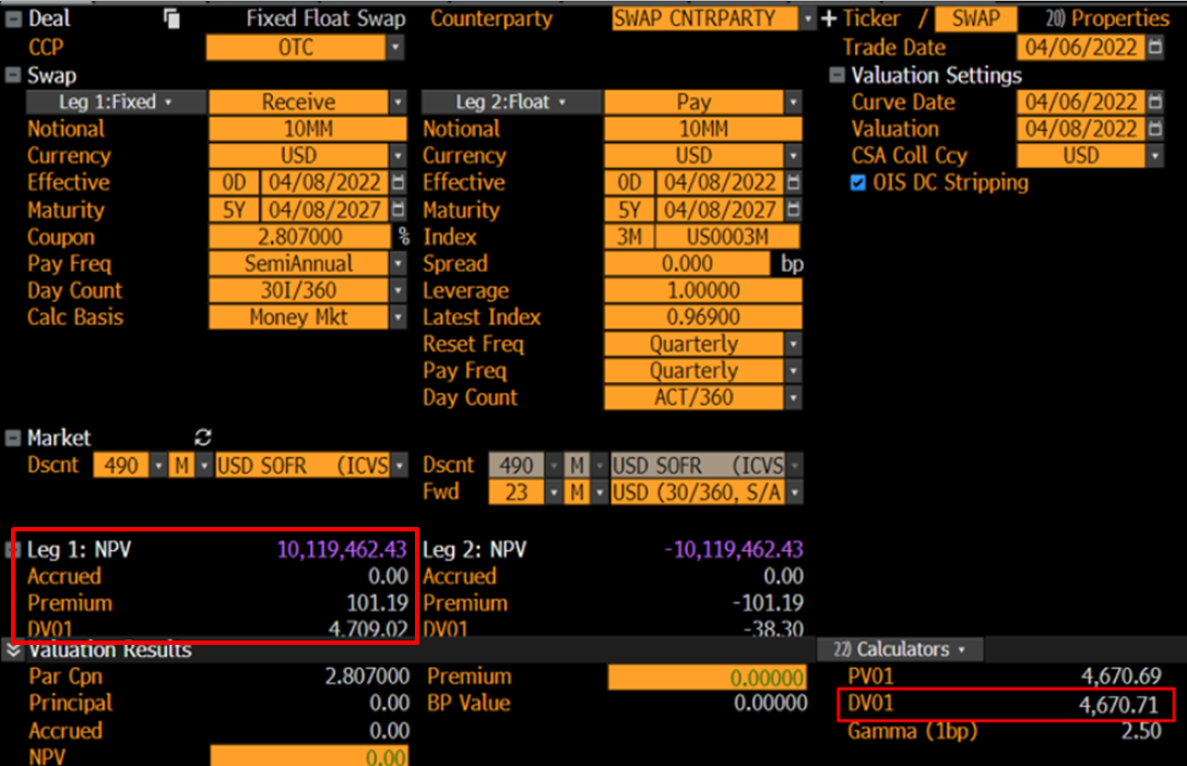
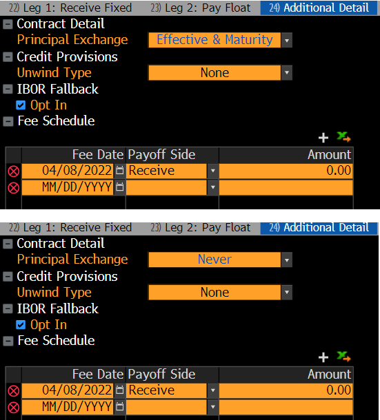
Assuming a standard FXFL USD 3m Libor (same outcome for EUR or USD SOFR though), if you have Details – Additional Detail – principal exchange set to the default "Effective and Maturity" (or pretty much anything except Never), you get the DV01 on the fixed leg. enter image description here
enter image description here

You can replicate DV01 in the scenario tab. Make sure you shift all curves - one scenario with -10bps, the other +10bps. enter image description here
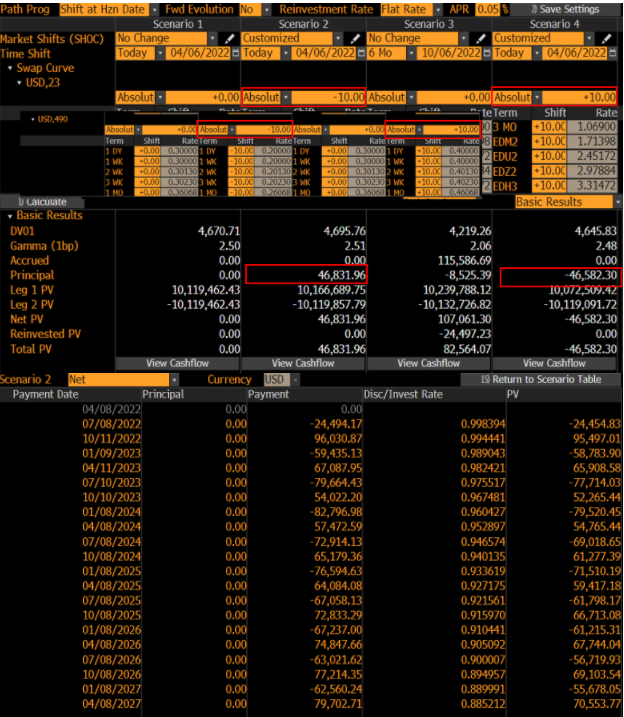
The cashflows in the screenshot can be seen by clicking on view Cashflow. We can compute this in Python like so:

down_net_PE = (-24454.83,95497.01,-58783.90,65908.58,-77714.03,52265.44,-79520.45,54765.44,-69018.65,61277.39,-71510.19,59417.18,-61798.17,66713.08,-61215.31,67744.04,-56719.93,69103.54,-55678.05,70553.77)
up_net_PE = (-24442.50,90152.58,-63632.96,60762.28,-82381.46,47178.37,-84696.57,46072.23,-73548.68,56223.43,-75730.07,54690.73,-66002.74,61679.37,-65255.04,62888.32,-60684.76,64056.32,-59536.51,65625.37)
print(f'Principal Down shift 10bps = {round(sum(down_net_PE),2)}')
print(f'Principal Up shift 10bps = {round(sum(up_net_PE),2)}')

DV01_PE = (sum(down_net_PE) - sum(up_net_PE))/20
print(f'DV01_PE = {round(DV01_PE,2)}')

The result is:

enter image description here

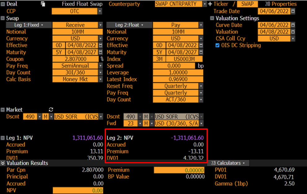
If you set principal exchange to never, you get this picture, where DV01 largely moves to the float leg:
enter image description here

You can get all casfhlows:

down1_pe = (
141895.94,
137882.74,
135031.58,
132253.10,
131947.95,
130129.08,
128556.34,
127029.73,
125607.28,
8976356.00
)

down2_pe = (
-24454.83,
-46398.93,
-58783.90,
-71974.16,
-77714.03,
-82766.14,
-79520.45,
-77487.65,
-69018.65,
-70670.56,
-71510.19,
-70711.90,
-61798.17,
-61843.27,
-61215.31,
-59285.69,
-56719.93,
-56503.73,
-55678.05,
-8905802.2
)

down1 = (
141895.94,
137882.74,
135031.58,
132253.10,
131947.95,
130129.08,
128556.34,
127029.73,
125607.28,
124239.47

)

down2 = (
-24454.83,
-46398.93,
-58783.90,
-71974.16,
-77714.03,
-82766.14,
-79520.45,
-77487.65,
-69018.65,
-70670.56,
-71510.19,
-70711.90,
-61798.17,
-61843.27,
-61215.31,
-59285.69,
-56719.93,
-56503.73,
-55678.05,
-53685.70
)

up1 = (141750.28,
137606.33,
134626.59,
131728.62,
131294.15,
129356.92,
127667.00,
126026.87,
124492.60,
123016.01
      )

up2 = (
-24442.50,
-51597.70,
-63632.96,
-76844.06,
-82381.46,
-87448.22,
-84696.57,
-85656.39,
-73548.68,
-75070.72,
-75730.07,
-74666.20,
-66002.74,
-65987.64,
-65255.04,
-63138.56,
-60684.76,
-60436.28,
-59536.51,
-57390.63
)

up1_pe = (141750.28,
137606.33,
134626.59,
131728.62,
131294.15,
129356.92,
127667.00,
126026.87,
124492.60,
8887960.04
      )

up2_pe = (
-24442.50,
-51597.70,
-63632.96,
-76844.06,
-82381.46,
-87448.22,
-84696.57,
-85656.39,
-73548.68,
-75070.72,
-75730.07,
-74666.20,
-66002.74,
-65987.64,
-65255.04,
-63138.56,
-60684.76,
-60436.28,
-59536.51,
-8822334.6
)

where _pe denotes with principal exchange (only difference is last value) and the number refers to the respective leg of the swap.
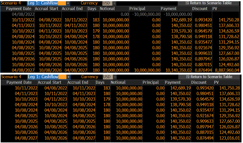
enter image description here

enter image description here

Manually computing the DV01's results in: enter image description here
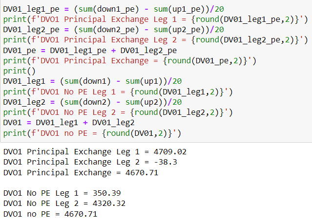
Which is identical to SWPM. The help page has a fairly lengthy explanation of the setting for Libor fixing. In a nutshell, the only difference is the first cashflow. enter image description here
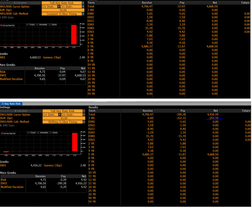
4668.53 - 252.31 = 4416.22

It does affect the DV01 on the main tab, but not the one in the Greeks section of the Risk tab. While stripping ICVS curves, the fixed first Libor rate is used. Hence, the choice for Libor fixing only affects sensitivity calculations.

If you are worried that the curves are designed from heterogeneous market instruments (Cash rate, Futures / FRAs, Par Swaps), you can use the Risk tab to define shifts on homogenous curves: if you shift Forwards (essentially assuming the curve is solely constructed using forward rates /FRAs), shift swaps (assuming only par swaps are used in curve construction), shift zeros.

Bottom line:

  • BBG shifts also the discounting curve and does not leave it untouched
  • If you want to be consistent with the way the swap curves are designed by default (and swaps are priced in BBG), you should shift the curve instruments and use constant libor. This should also be the swap defaults as defined in SWDF DFLT.
$\endgroup$
1
$\begingroup$

Since I do not have Bloomberg I can only give a general comment.

Ingoring for simplicity the fact that we now have different curves for discounting and projecting forward floating rates, LIBOR basis and what not, the PV of the floating leg of the swap is $$\tag{1} {\rm PV}_{\text{float}}=1-P(0,T_n) $$ (assuming again for simplicity that the swap starts today and $P(0,T_n)$ is the discount factor from the swap maturity $T_n$). Likewise, the PV of the fixed leg is $$\tag{2} {\rm PV}_{\text{fix}}=\sum_{i=1}^n CP(0,T_i) $$ where $C$ is the fixed rate in the swap. Assuming for simplicity annual payments.

Theoretically, the interest rate risk of the swap is obtained by shifting each rate that was used to construct the discount factors $P(0,T_i)$ then revaluing the swap and then taking the PV difference.

What Bloomberg seems to do instead is to calculate the new fixed PV by shifting the fixed rate $C$. Even though it stays constant (it is a term of the trade) this is approximately valid because when all rates change that were used to construct the discount factors then in particular the fair swap rate for maturity $T_n$ will change. This fair swap rate is related to the discount factors by $$ C_{\text{fair}}=\frac{1-P(0,T_n)}{\sum_{i=1}^n P(0,T_i)} $$ which follows simply from ${\rm PV}_{\text{float}}={\rm PV}_{\text{fix}}$.

In practice it turns out that $C_{\text{fair}}$ changes a lot more than the individual discount factors do. Therefore, in practice it is a good assumption that

  • ${\rm PV}_{\text{float}}$ doesn't change

  • ${\rm PV}_{\text{fix}}$ changes by the ${\rm DVO1}(T_n)$ because \begin{align} {\rm PV}_{\text{fix}}'-{\rm PV}_{\text{fix}}&=\sum_{i=1}^n C'_{\text{fair}}P(0,T_i)- \sum_{i=1}^n C_{\text{fair}}P(0,T_i)\\ &=\sum_{i=1}^n \underbrace{(C_{\text{fair}}'-C_{\text{fair}})}_{\text{ typically 1 or 10 bps}} P(0,T_i)={\rm DVO1}(T_n)\,. \end{align} This is applicable to $C$ as well if we assume that this changes by the same amount as the swap rates are changing that are used to build the discount factors.

$\endgroup$
2
  • 1
    $\begingroup$ "What Bloomberg seems to do" without lookig at the terminal, are you sure? $\endgroup$ Commented May 23, 2022 at 12:16
  • $\begingroup$ If I was I would have written: "what BBG does". $\endgroup$
    – Kurt G.
    Commented May 23, 2022 at 12:21
1
$\begingroup$

Just a point of clarification in relation to the "OIS discounting curve" and the "par swap curve". The question is somewhat confusing because it seems to imply that these are disjointed "ingredient curves" and go into the valuation (of e.g. a Libor fix-float swap). The OIS discounting curve is actually used to construct the par swap rate curve itself (i.e. to compute the Libor forward rates of the par swap curve). The par swap curve sensitivity impacts the Libor forwards directly. The discounting curve sensitivity also impacts the Libor forward rates (and the hence the par swap curve), albeit indirectly. In this sense the two curves (and their sensitivities) are intertwined. While previous answers demonstrate that it's possible to distinguish between their independent sensitivities, it's important to keep this interdependence in context.

$\endgroup$

Your Answer

By clicking “Post Your Answer”, you agree to our terms of service and acknowledge you have read our privacy policy.

Not the answer you're looking for? Browse other questions tagged or ask your own question.