I am trying to simulate $n$ correlated geometric brownian motions (GBM) given a specified correlation matrix $\Sigma$ by following this procedure which uses Cholesky decomposition.
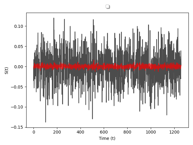
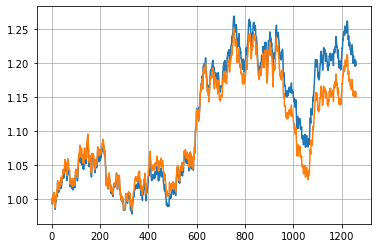
However, when I implement the code in Python one of the highly correlated ($\rho=0.99$) Wiener Processes have almost no volatility as can be seen in the plot below in the red line.
I would expect a correlation of $\rho=1$ to imply that the two processes would be identical and for $\rho=-1$, I would expect a "mirror" around 0.
The plot shows the realization of $W$ across $t$.
Note: In my attempt I try to avoid using any loops.
# PARAMETERS
n = 2                                              # number of assets
T = 5                                              # number of years
N = 252                                            # number of steps pr. year (T)
r = np.array([0.03, 0.03])                         # drift-rate
q = np.array([0.0, 0.0])                           # divivend-rate
S0 = np.array([1.0, 1.0])                          # initial value
sigma = np.array([0.2, 0.2])                       # diffusion-coefficients
corr_mat = np.array([[1.0, 0.99], [0.99, 1.0]])    # correlation-matrix

# Calculate step size
dt = 1 / (T * N)

# Vector of time index
t = np.array(range(N*T+1)).reshape((N * T + 1, 1)) * dt


# == PERFORM SIMULATION ==
# Draw normal distributed random variables
eps = np.random.normal(loc=0, scale=np.sqrt(dt), size=(N * T, n))


# Use Cholesky decomposition to get the matrix R satisfying: corr_mat = L x L^*
L = np.linalg.cholesky(corr_mat)

# Transform into realizations of correlated Wiener processes
W = eps @ L

# Calculate realizations of each stock as the realization of a GBM
# S_t = S0 * exp{ ((r-q) - ½sigma)*dt + sigma * W}
S = np.exp(
    (((r - q) - np.power(sigma, 2) / 2) * dt).T + W * sigma.T
)
S = np.vstack([np.ones(S.shape[1]), S])
S = S0 * S.cumprod(axis=0)


