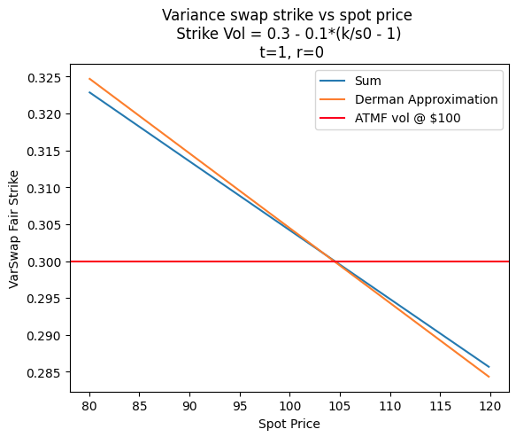
The fair strike computed via replication equals the integral of weighted prices of out-of-the-money options over all strikes. As you wrote correctly, these weights are being inversely proportional to squared strikes, an application of the Black Scholes closed-form formula for gamma, which ensures results in constant dollar gamma.
In your example, the OTM options changed with the change in ATMS. Since your prices for OTM options (and ATM) are different now for every weight, you should end up with a different variance swap strike.
In what follows, I'll rely heavily on the excellent answers given to this question. The par rate (or variance swap strike) is defined as (copied from @Quantuple in the linked question):
$$ K_{var} = \frac{2}{B(0,T)T} \left[ \int_0^{F(0,T)} \frac{P(K,T)}{K^2} dK + \int_{F(0,T)}^\infty \frac{C(K,T)}{K^2} dK \right] $$
where $T$ is the contract's maturity date, $B(0,T)$ the discount factor, $P(K,T)$ and $C(K,T)$ European option prices with strike $K$ and maturity $T$ and $F(0,T)$ the forward price. There are two documents from JP Morgan Variance Swaps and Just what you need to know about Variance Swaps that contain the formula and details, with the latter being more concise. Personally, I recommend reading Towards a Theory of Volatility Trading by Peter Carr et al.
I'll express the variance strike as $\sqrt{K_{var}}\times 100$. Moreover, I assume dividends and interest rates are zero to skip discounting and to simplify the formula somewhat because ATMS = ATMF.
The Julia equivalent code of @will's answer, made interactive and suitable for your question, looks like this:
 # load packages
using Distributions, Plots ,DataFrames, Interact,Plots, PlotThemes, QuadGK
N(x) = cdf(Normal(0,1),x)

# generic put call pricer (cp = call_put_flag, 1 = call -1 = put)
function BSM(S,K,t,rf,d,σ, cp)
    d1 = ( log(S/K) + (rf - d + 1/2*σ^2)*t ) / (σ*sqrt(t))
    d2 = d1 - σ*sqrt(t)
    opt  = cp*exp(-d*t)S*N(cp*d1) - cp*exp(-rf*t)*K*N(cp*d2)
  return opt
end

# compute vol surface
function vols(k, vol_atm, convexity, skew, s)
    v = 0.5*convexity*k^2 + (skew - convexity*s)*k + vol_atm + 0.5*convexity*s^2 - skew*s
    return v
end

# create interactive chart
@manipulate for ATM=0.0:0.01:0.5, Skew=-0.001:0.0001:0.001, Convexity=-0.0001:0.00005:0.0005, s1 = 10:1:90, s2 = 12:1:92  ;
    atm_vol,convexity, skew, ks, T, r,d = ATM, Convexity, Skew, 10:1;80, 1, 0,0
    IVs = [vols(k, atm_vol, convexity, skew, S1) for k in ks]
    inputs = ks .=> IVs
    res1 = [BSM.(s1,k,T,r,d,vols(k, atm_vol, convexity, skew, s1), k < s1 ? -1 : 1).* k^-2 for k in ks]
    res2 = [BSM.(s2,k,T,r,d,vols(k, atm_vol, convexity, skew, s1), k < s2 ? -1 : 1).* k^-2  for k in ks]

    # compute fair VS strike as the integral of OTM calls and put options
    vs_strike1 = round(100*sqrt(2*(quadgk(k -> BSM.(s1,k,T,r,d,vols(k, atm_vol, convexity, skew, s1), -1)* k^-2, 0, s1)[1] + quadgk(k -> BSM.(s1,k,T,r,d,vols(k, atm_vol, convexity, skew, s1), 1)* k^-2, s1,150)[1])) , digits = dig)
    vs_strike2 = round(100*sqrt(2*(quadgk(k -> BSM.(s2,k,T,r,d,vols(k, atm_vol, convexity, skew, s1), -1)* k^-2, 0, s2)[1] + quadgk(k -> BSM.(s2,k,T,r,d,vols(k, atm_vol, convexity, skew, s1), 1)* k^-2, s2,150)[1])) , digits = dig)
    p2 = plot([k for (k,v) in inputs], [v for (k,v) in inputs], label = "Vol Surface", xlabel = "Strikes", ylabel = "IV")
    vline!([s1], label = "ATMS = $(s1) with IV = $(round(vols(s1, atm_vol, convexity, skew, s1), digits =4))")
    vline!([s2], legendposition = :topright, label = "ATMS = $(s2) with IV = $(round(vols(s2, atm_vol, convexity, skew, s1), digits = 4))")
    p1 = plot(ks, res1, size=(950,700), left_margin=3Plots.mm, label =  "ATM Spot = $(s1) => Fair VS Strike = $(vs_strike1)", title = "Weighted (1/K^2) OTM Put and Call Options")
    plot!(ks, res2, label = "ATM Spot = $(s2) => Fair VS Strike = $(vs_strike2)", xlabel = "Strikes")
    vline!([s1], label = "ATMS = $(s1) with IV = $(round(vols(s1, atm_vol, convexity, skew, s1), digits =4))")
    vline!([s2], legendposition = :bottomleft, label = "ATMS = $(s2) with IV = $(round(vols(s2, atm_vol, convexity, skew, s1), digits = 4))")
    plot(p1,p2, layout = (2,1) )
    end
Explanation:
- BSM is standard Black Scholes Merton, with the last input defining call (1) and put (-1)
- The code uses a simple functional form to create a vol surface that exhibits skew and curvature
- s1 refers to the original ATMS and ATM vol as defined by the surface logik refers to this spot value
- The area under the weigthed prices is the fair VS strike, which is computed using package called QuadGK, which applies a numerical integration scheme using an adaptive Gauss-Kronrod integration technique: the integral in each interval is estimated using a Kronrod rule (2*order+1 points) and the error is estimated using an embedded Gauss rule (order points). The interval with the largest error is then subdivided into two intervals and the process is repeated until the desired error tolerance is achieved.
Result:
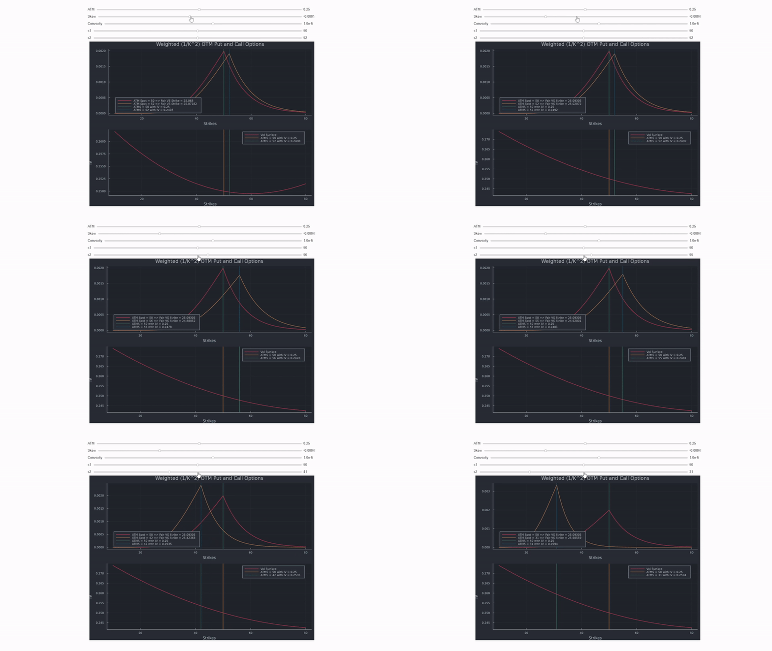
Keeping the vol surface, while moving along the skew will lead to different OTM option prices and different VS strikes as can be seen in the GIF below.

Because the quality of the GIF is not great (size limit of imgur), I also include a screenshot:

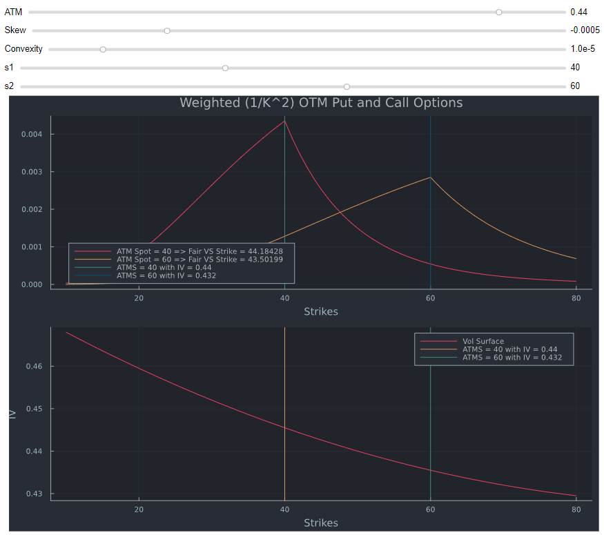
You can find a more detailed chart that highlights the area under the OTM options here. The chart can also be used to show that skew is less important compared to convexity because the fair VS strike becomes larger relative to the ATM level.
Side remark, due to practical difficulties in replicating the actual log payout across strikes, the market for equity index varswaps usually trades at a basis to the replicating portfolio.

