The T+H Problem in Factor model forecasts

Question

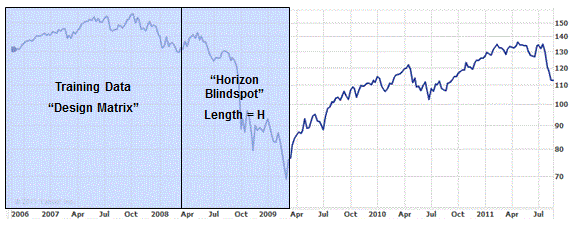
Suppose we train on M individuals consisting of T observations (i.e. TxM design matrix). The dependent variable is one-year return for each security (H = horizon of one year). In a factor model specification, we align security characteristics and economic factor exposures observed at time T with the dependent variable observed at T+H. Therefore any operational forecasting factor model must use information that is stale by at least one-year.

This can have traumatic consequences especially as market conditions are continuously changing. For example, such a forecasting model would not “recognize” a bear market until at least one full year into the bear market (maybe when the bear market ended as in the illustration below). Likewise, a full one year after the end of the bear market on March 2009 such a forecasting model would continue to predict substantial negative returns thru March 2010 and then some. Or consider today -- a 1 year forecasting model’s most recent training data is an observation from August 2010 – changes in factor premia are lagged by construction.

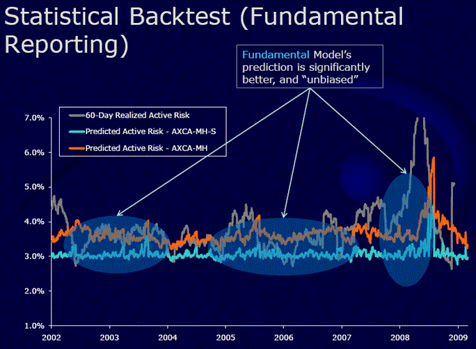
Check out this slide from an Axioma Risk Model presentation:

Notice the lagged "echo" volatility spike that takes place months after October 2008 -- several months after the realized volatility spike. Perversely, as realized risk (gray line) is declining the predicted risk (red/blue line) is increasing! This is because the realized volatility enters the training data with some lag. There is no "instantaneous" adjustment to current conditions.

What creative work-arounds or modeling approaches can be used to dealing with this problem endemic to forecasting models? Are there statistical methods to cope with this?

Answer 1

I can offer three suggestions:

(a) Since any model, however sophisticated, will miss tail cases (such as Oct 2008) I would increase the number of high-frequency factors (eg weekly jobless claims - I don't know if that is a relevant example in your case - but just to give you an idea) in the model. Not only does that make the model more responsive to current events, it would also allow the H-window to be shortened while still maintaining a low variance for model error (as sample size within a time window remains unaffected)

(b) Weighting, maybe? Give more weightage to recent points and lesser so to older data. Some HVaR models I have seen do apply this while still giving tail events a higher weightage (manually) - thus maintaining predictive capacity for tail events (which we are more concerned about, anyway) while making the model less "burdened" by older, redundant data (not all data adds "new" information).

(c) Some sort of instantaneous feedback to calculate how "off" your model is. The larger this "difference" metric is, the more intensely you can apply your weighting rules as described in (b). This again makes the model more responsive to volatile current events.

Answer 2

Hopefully these ideas open up some solution strategies.

A. Calibration approach: In the case of a volatility model such as Axioma's above, you could perform an instantaneous volatility adjustment. Procedure:

1. You build your usual T+H volatility model.
2. You measure the realized volatility and implied volatility of the training set.
3. You measure the out-of-time performance your T+H volatility model (specifically, realized volatility and implied volatility) over some period.
4. You identify a scaling factor that is a function of the observed volatility today and the implied and realized volatility of the training set. For example, imagine that the out-of-time realized volatility was 2x the volatility of your training set. Then a naive scaling factor of 2x can be applied to your covariance matrix -- of course you can do better by estimating the relationship.

Weakness: The above procedure might work for volatility estimation where you have one dependent variable or one covariance matrix that you scale up or down. But it's not clear how you would apply this to a cross-sectional equity return model.

B. Regime Switching Model: Another approach would be to setup a regime switching model. Here you are conditioning returns and volatility expectations on today's state. You estimate the expected returns and volatility associated with each state. This is an improvement in that you are making use of today's states but you still have a subtle T+H problem since the dependent variable is still lagged. Also, your model will have difficulty handling regimes not in the training set such as stagflation, QE3, etc. and you have the usual issues with regime models (parameter estimation, new regimes, convergence, etc.). This approach has the most merit in asset allocation policy and volatility estimation.

C. Forecast for half-the horizon. This is a bit like Zeno's paradox though -- why not forecast for half of half of the horizon? Another drawback is that different correlation structures emerge at different time scalings.

D. One angle would be a hybrid model. Estimate the contemporaneous factor returns and then have another model that forecasts the evolution of each factor. Weakness here is the complexity -- you go from one model to K+1 models (one model for each factor). You are estimating too many parameters with the same data.

E. Weighting + Re-scaling. Here you take a some rolling average of exponentially weighted factor returns and scale them to an annualize horizon and add to your training set. Problem is you would get unrealistic data. For example, if you had 4 consecutive weeks of sub-par returns you would extrapolate a correction into financial armageddon.

(B) is no panacea but it seems like the most promising approach. To my knowledge BARRA, Axioma, et al do not apply regime switching models. What other techniques might we be missing?