target market correlation for long / short equity portfolio

Question

Given a long / short equity portfolio, I want to have some net long market exposure.

My portfolio volatility is fixed to a target, so I don't think it makes sense to target market beta. I think I have to target my correlation to the market.

Does it make sense to get market exposure by targeting correlation? If so, how can I accomplish this? Potentially relevant quantities:

• Correlation matrix of portfolio stocks to each other
• Time series of rolling correlations of stocks to the market
• Time series of rolling volatility estimates of stocks
• Time series of rolling volatility estimates of market

Also, I should note that the long side tends to have low beta stocks and the short side has high beta stocks, so it isn't sufficient to use dollar exposure to manage market exposure.

Answer 1

Portfolio beta is a function of market vol, portfolio vol and correlation between market and portfolio; so correlation is indeed the only free variable. (But if you have complete control over the portfolio-construction process, you might as well target beta and then scale the weights so that you meet your volatility target.)

To control correlation, you'll need a forecast of correlation first, and different setups for getting these forecasts -- e.g. using historical data with shrinkage, specific time horizons, etc -- may give different results. What works well is an empirical question, but given that correlations are notoriously unstable, you should not expect to be able to fine-control correlation out-of-sample. In any case, eventually, these forecasts are put into a correlation matrix (allowed assets + market).

If your portfolio was created via a optimization model, you may add correlation directly, as a target or as a restriction. Alternatively, you could create an overlay model, whose aim is to maximize correlation subject to a restriction on how much change to the portfolio you would be willing to allow.

---

Update, following the comment: They way I suggest to handle this is via a direct optimization of correlation. All you then need is an optimization algorithm that is capable of solving such models. Heuristics, for instance, can handle such models (see Heuristic Optimisation in Financial Modelling or Heuristics for Portfolio Selection). Whether a particular model make sense empirically is a, well, empirical question; but the computation is quite straightforward. Let me sketch an example, using R, for the 'overlay' approach. I'll keep this example very simple.

Suppose you have a set R of return scenarios of your assets. Every column hold the return of one asset. I also create a 'market' time-series, M. For simplicity, I use historical data here. The data set consists of 48 industry portfolios provided by Kenneth French (I drop the other industry.)

library("NMOF")        ## https://github.com/enricoschumann/NMOF
library("neighbours")  ## https://github.com/enricoschumann/neighbours

R <- French("~/Downloads/French",
            "49_Industry_Portfolios_daily_CSV.zip")
R <- R[seq(to = nrow(R), length.out = 500), 1:48]
R <- as.matrix(R)

M <- French("~/Downloads/French",          
            dataset = "market",
            frequency = "daily")

all(row.names(R) %in% row.names(M)) ## check
## [1] TRUE

M <- M[row.names(R), ]
M <- as.matrix(M)

I create a random original portfolio. It is a zero-investment portfolio, with fairly large weights.

orig.portfolio <- runif(ncol(R), min = 0, max = 0.3)
orig.portfolio <- orig.portfolio - mean(orig.portfolio)

summary(orig.portfolio)
##     Min.  1st Qu.   Median     Mean  3rd Qu.     Max. 
## -0.15474 -0.07257  0.02445  0.00000  0.06513  0.12166 

round(sum(orig.portfolio), 8)
## [1] 0

The goal is now to create a zero-investment overlay, with maximum deviations of -0.025 to 0.025, say, that maximizes the correlation with the market M. The objective function cr is straightforward. We later minimize, so I put a minus in front of the correlation.

cr <- function(x, orig.portfolio, R, M)
    -c(cor(R %*% (x + orig.portfolio), M))

## cor(R %*% (orig.portfolio), M)
-cr(0, orig.portfolio, R, M)
## [1] 0.04762037

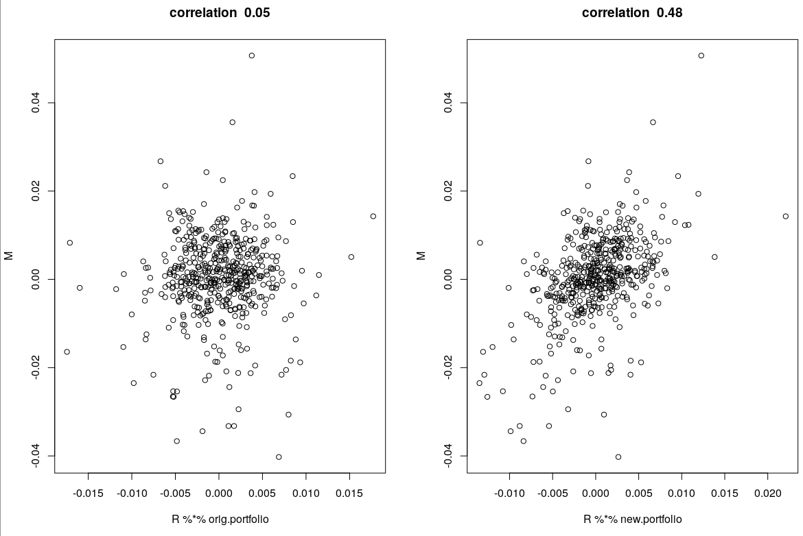
So the original portfolio had a correlation of 0.05. Now I minimize the function, using a method called Threshold Accepting.

nb <- neighbourfun(min = -0.025, max = 0.025, stepsize = 0.005)
sol <- TAopt(cr,
             list(nI = 10000,
                  x0 = c(0.01,-0.01, rep(0, ncol(R)-2)),
                  neighbour = nb),
             orig.portfolio = orig.portfolio,
             M = M,
             R = R)

-cr(sol$xbest, orig.portfolio, R, M)
## [1] 0.4776

So the new portfolio, which is still zero-investment, has a correlation of 0.48. For simplicity, I scale the new portfolio so that it has the same volatility as the original one. This will not affect the correlation.

new.portfolio <- orig.portfolio + sol$xbest
new.portfolio <- new.portfolio/sd(R %*% new.portfolio)*sd(R %*% orig.portfolio)
sd(R %*% orig.portfolio)
## [1] 0.004195
sd(R %*% new.portfolio)
## [1] 0.004195

-cr(new.portfolio-orig.portfolio, orig.portfolio, R, M)
## [1] 0.4776

We may also plot the portfolio returns under the scenarios R. On the left, the original portfolio; on the right, the portfolio with the overlay.

par(mfrow = c(1, 2))
plot(R %*% orig.portfolio, M,
     main = paste("correlation ",
                  round(-cr(0, orig.portfolio, R, M), 2)))
plot(R %*% new.portfolio, M,
     main = paste("correlation ",
                  round(-cr(new.portfolio-orig.portfolio, orig.portfolio, R, M), 2)))

(Disclosure: I am the maintainer of R packages used in the examples, and a coauthor of the papers I suggested above.)