Efficient frontier doesn't look good

Question

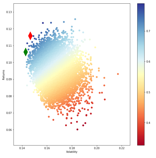
Hi I'm trying to draw an efficient frontier. Below is what I used. returns parameter consists of 9 column returns of portfolio. I selected 10,000 portfolios and this is how my efficient frontier looked like. This is not the usual frontier shape that is familiar to us.

Data set is 48_Industry_Portfolios_daily.csv, obtained from (http://mba.tuck.dartmouth.edu/pages/faculty/ken.french/data_library.html). The first 9 columns were selected

Can somone kindly explain me the issue.

def portfolio_annualised_performance(weights, mean_returns, cov_matrix):
    returns = np.sum(mean_returns*weights ) *252
    #print ('weights shape',weights.shape)
    #print (' Returns ',returns)
    std = np.sqrt(np.dot(weights.T, np.dot(cov_matrix, weights))) * np.sqrt(252)
    #print ('Std ',std)
    return std, returns

def random_portfolios(num_portfolios, mean_returns, cov_matrix, risk_free_rate):
    results = np.zeros((3,num_portfolios))
    weights_record = []
    for i in range(num_portfolios):
        weights = np.random.random(48)

        weights /= np.sum(weights)
        weights_record.append(weights)
        portfolio_std_dev, portfolio_return = portfolio_annualised_performance(weights, mean_returns, cov_matrix)
        results[0,i] = portfolio_std_dev
        results[1,i] = portfolio_return
        results[2,i] = (portfolio_return - risk_free_rate) / portfolio_std_dev
    return results, weights_record

def monteCarlo_Simulation(returns):

    #returns=returns.drop("Date")
    returns=returns/100
    stocks=list(returns)
    stocks1=list(returns)
    stocks1.insert(0,"ret")
    stocks1.insert(1,"stdev")
    stocks1.insert(2,"sharpe")
    print (stocks)
    #calculate mean daily return and covariance of daily returns
    mean_daily_returns = returns.mean()
    #print (mean_daily_returns)
    cov_matrix = returns.cov()

    #set number of runs of random portfolio weights
    num_portfolios = 10000


    #set up array to hold results
    #We have increased the size of the array to hold the weight values for each stock
    results = np.zeros((4+len(stocks)-1,num_portfolios))

    for i in range(num_portfolios):
        #select random weights for portfolio holdings
        weights = np.array(np.random.random(len(stocks)))
        #rebalance weights to sum to 1
        weights /= np.sum(weights)

        #calculate portfolio return and volatility
        portfolio_return = np.sum(mean_daily_returns * weights) * 252
        portfolio_std_dev = np.sqrt(np.dot(weights.T,np.dot(cov_matrix, weights))) * np.sqrt(252)

        #store results in results array
        results[0,i] = portfolio_return
        results[1,i] = portfolio_std_dev
        #store Sharpe Ratio (return / volatility) - risk free rate element excluded for simplicity
        results[2,i] = results[0,i] / results[1,i]
        #iterate through the weight vector and add data to results array
        for j in range(len(weights)):
            results[j+3,i] = weights[j]

    print (results.T.shape)
    #convert results array to Pandas DataFrame
    results_frame = pd.DataFrame(results.T,columns=stocks1)

    #locate position of portfolio with highest Sharpe Ratio
    max_sharpe_port = results_frame.iloc[results_frame['sharpe'].idxmax()]
    #locate positon of portfolio with minimum standard deviation
    min_vol_port = results_frame.iloc[results_frame['stdev'].idxmin()]

    #create scatter plot coloured by Sharpe Ratio
    plt.figure(figsize=(10,10))
    plt.scatter(results_frame.stdev,results_frame.ret,c=results_frame.sharpe,cmap='RdYlBu')
    plt.xlabel('Volatility')
    plt.ylabel('Returns')
    plt.colorbar()
    #plot red star to highlight position of portfolio with highest Sharpe Ratio
    plt.scatter(max_sharpe_port[1],max_sharpe_port[0],marker=(2,1,0),color='r',s=1000)
    #plot green star to highlight position of minimum variance portfolio
    plt.scatter(min_vol_port[1],min_vol_port[0],marker=(2,1,0),color='g',s=1000)

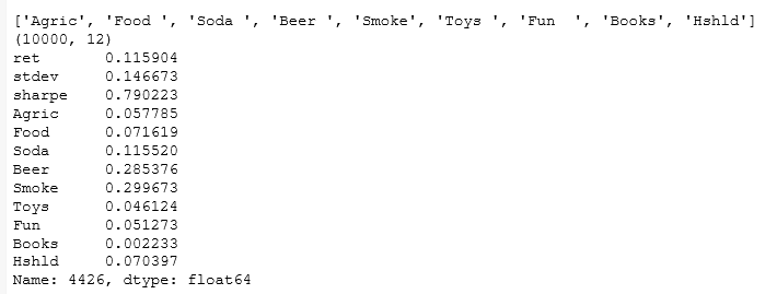
    print(max_sharpe_port)

updated answer

Also I'm asked to compare portfolio variance using different regularizes and to use a validation methods to find the optimal parameters. Can we use python to do this?

Answer 1

As i understand your question you are confused as to why the expected parabola-shape of the frontier is not depicted clearly.

If you want to see the shape more clearly you can do one of two things:

1. Increase the number of random portfolios. As this numbers goes to infinity you will eventually plot all possible portfolio combinations, and your efficient frontier will be very visible.

2. Use the fact that all portfolios on the efficient frontier can be constructed by combinations of just two efficient portfolios (e.g. the max sharpe and the min. variance portfolios). You would do this by just constructing an array of portfolios ((return, std. dev)-pairs) with weights equal to $weights=w*\pi_{max}+(1-w)*\pi_{min}$ for an interval of $w$'s.

Instead of making 10,000 random portfolios to find the tangency and min.var. portfolios, you could also just solve for them using the equations

$$ \mathbf{\pi}_{\max SR} = \frac{1}{\mathbf{1'\Sigma^{-1}\mu}} \mathbf{\Sigma^{-1}\mu}$$

$$ \mathbf{\pi_{\min Var}} = \frac{1}{ \mathbf{1' \Sigma^{-1}1}} \mathbf{ \Sigma^{-1}1}$$

Where $\mathbf{\Sigma^{-1}}$ is the inverse of your variance-covariance matrix, $\mathbf{\mu}$ is your vector of expected returns, and $\mathbf{1}$ is a vector of 1's with the same length as your $\mathbf{\mu}$.

Answer 2

The reason why the efficient frontier doesn't look good is because It's not the efficient frontier. It's the feasible set.

What your code is doing is generating random portfolios, and plugging these random weight vectors as inputs into the formula of the mean-variance model. These random portfolios, when transformed like this to mean-variance coordinates, only provide the feasible set, which are portfolios inferior to the efficient frontier (seen as everything in the cloud to the right of the left boundary), and by chance many portfolios very close to or along the efficient frontier if you generate a high enough number of them. But it is not the direct way to solve for the efficient frontier, separate from the feasible set.

In order to plot the efficient frontier, you have solve for optimal portfolios along the efficient frontier directly, which requires convex optimization on the mean-variance model's formula,

$$\min_w w^\top \Sigma w \enspace \hspace{2cm} \text{s.t.} \enspace w^\top \mu = \theta, \enspace \sum_{i=1}^N w_i=1 $$

Optimizing the above formula with an optimizer for varying levels of target return $\theta$ will result in an optimal weight vector as an output. As you can tell, this procedure is not the same as plugging in random weights as inputs into the same formula as is done in the random portfolios approach.

In summary, you are currently doing the first of the following two approaches,

Random portfolios:

• use randomly generated weights as inputs for the mean-variance formula
• All solutions are only feasible portfolios (and if some are efficient portfolios, it is by chance)

Optimized portfolios:

• use mean-variance model itself to solve for optimal weights as outputs
• All solutions are efficient portfolios

Following approach 1 explains the high number of portfolios appearing in the far right, creating a circular cloud, being the feasible set, at such a high asset number size (48), which the other comments have pointed out happens by nature. Lowering the portfolio size (10 or lower), regardless if this is what you want, is the only way to reduce the number of 'outlying' feasible portfolios appearing in the far right of the feasible set if you insist on approach 1's usage (feasible, random portfolios) rather than approach 2 (efficient, optimized portfolios).

Answer 3

Whilst this doesn't answer your question you may be interested to know that you can vectorise your simulation and greatly improve the efficiency of your code like this:

def portfolio_annualised_performance(weights, mean_returns, cov_matrix):
    """
    Return annualised risk and return for a portfolio given asset weights and expected return and covriance

    Args:
        weights (ndarray): asset weights
        mean_returns (ndarray): expected returns of each asset
        cov_matrix (ndarray): covariance metrix of asset returns

    Returns:
        tuple: annualised risk (np.float64), annualised total return (np.float64)

    Notes:
        If weights is supplied as a 2D array, then outputs are not floats but 1D arrays.
    """
    return (np.sqrt(np.einsum('...i,ij,...j->...', weights, cov_matrix, weights) * 252),
            np.einsum('...i,i->...', weights, mean_returns) * 252)

def random_portfolios(size, mean_returns, cov_matrix, risk_free_rate):
    """
    Simulates a number of portfolio through random weights and calculates performance metrics

    Args:
        size (int): number of simulations
        mean_returns (ndarray): expected returns of each asset
        cov_matrix (ndarray): covariance metrix of asset returns
        risk_free_rate (np.float64): annualised risk free return

    Returns:
        tuple: annualised risk (ndarray), annualised total return (ndarray), Sharpe ratio (ndarray), weights (ndarray)
    """
    rand_weights = np.random.random(size=(size*mean_returns.shape[0])).reshape(size, -1)
    rand_weights /= np.sum(rand_weights, axis=1)[:, np.newaxis]
    perf = portfolio_annualised_performance(rand_weights, mean_returns, cov_matrix)
    return perf + ((perf[1] - risk_free_rate)/perf[0], rand_weights)

Answer 4

This has occurred to me as well when trying to simulate the efficient frontier. The conclusion I came up with was the as I increase the number of instruments I try to use, the frontier losses its shape. If you want to check your code correctness, simply leave 2-3 instruments, see the results that come up, I'm quite sure you'll see the usual shape come up.

Answer 5

Since the first part of your question was already answered, I provide you with a solution for the second part "Also I'm asked to compare portfolio variance using different regularizes and to use a validation methods to find the optimal parameters. Can we use python to do this?"

You can do the regularization with 3 techniques: Ridge (the regulatization happens by adding the sum of the squared weights to the OLS part), Lasso(the regulatization happens by adding the norm 1 of the weights to the OLS part) and ElasticNet regressions(the regulatization happens by adding both the previous to the OLS part). To do this you need to code yourself this during the definition of your optimisation problem. To run such optmimisation you can use:

import cvxpy

This is the package for the convex optimisation. I do not report the mathematical formulation of the regularization as you can find tons of them on the web, I just want to mention that in Ridge and Lasso you need to estimate one parameter, while in the ElasticNet you need to estimate two because ElastcNet is a combination of Lasso and Ridge. This contribution must be added to the typical cost function wTCw to minimise.

For the estimation of the regularized parameter you need to apply cross validation. You can do it in python. You might think of using k-fold cross validation, but if you are dealing with time series data which have serial correlation it is not ideal as you may end up having correlated samples in test and training set, which can cause a misleading high R square.

So I suggest you to use a modified version of K-fold called Purged with Embargo k-fold cross validation. This was introduced by Lopez De Prado in his amazing "Advances in Financial Machine Learning". The basic idea is to make gaps between trainign and test sets while splitting them to reduce as much as possible the effect of serial correlation. To implement this new version of k-fold you need to make the class for it as it is not present in sklearn. But the book can help with this too.