Bergomi: Skew arbitrage

Question

In his paper "Smile Dynamics IV" (https://www.fields.utoronto.ca/programs/scientific/09-10/finance/derivatives/bergomi.pdf) as well as in his book "Stochastic Volatility Modeling" (Chapter 9.10) Lorenzo Bergomi proposes a "Skew Arbitrage Strategy". As I understand his logic, he is saying that for short maturities the skew stickiness ratio should be close to 2 (i.e. the implied ATM vol move for an dS_rel % spot move is 2 * Skew * dS_rel ). However, empirically the realised absolute spot move tends to be less than that, so one could buy a gamma neutral 1 month 95/105 risk reversal, delta hedge and hold it for one day. Since we are gamma neutral, as given by a Taylor expansion this position's PnL should be determined by

skew PnL + Vega PnL + "Mark to Market PnL"

"skew PnL" is proportional to realised spot vol covariance minus implied spot vol variance and will on average be positive as the realised stickiness is smaller than the implied one.

Vega PnL is small compared to the rest and basically just adds some noise.

"Mark to Market PnL" comes from recalibrating the vol model. More precisely, he is using a simple vol model, which is quadratic in log moneyness

$$\widehat{\sigma}(x)=\sigma_{0}\left(1+\alpha\left(\sigma_{0}\right) x+\frac{\beta\left(\sigma_{0}\right)}{2} x^{2}\right)$$

So each day, we would have to recalibrate the skew and curvature. In his book and paper Bergomi says that this Mark to Market PnL should be negligible. However, if I buy a 30 day option today, this will be a 29 day option tomorrow. The 95/105 skew decays (i.e. becomes more negative) as time to maturity goes down, so there should be a downward drift on the PnL. I tried to replicate the strategy and can indeed observe such a downward drift. It is smaller than the skew PnL, but has a non negligible effect on the PnL. In my replication I am using the S&P and my time period is 2010 to 2019, while Bergomi is using Eurostoxx and 2002-2010, so it is possible that I am picking up on a structural difference or a regime shift.

My questions are:

1. Is there some mistake in my thinking? Is it correct that there should be a PnL drift induced by the skew decay and that this is not necessarily small? Has anyone ever tried to simulate this for the S&P and made a similar observation? It is of course possible that I made a mistake.
2. It is not intuitively clear to me, why this strategy should only work for short maturity options. Basically all that is done to motivate it is to take a vol model quadratic in log moneyness and plug it into a Taylor expansion for the total option PnL. Where does this break down for, say a 90 day option, and is there a way to get something similar here?

Edit: Some additional observations

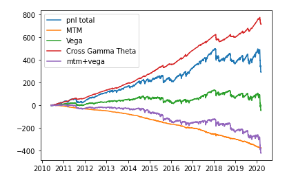
I am adding a plot with a decomposition for the PnL of the 35day 95/105 gamma neutral risk reversal for the S&P. Unfortunately I only have data until March 13 2020, so I am missing the interesting moves after this date. "PnL Total" is the PnL is the PnL of the position. "MTM" is the PnL from remarking the skew parameter and the quadratic ("vol of vol") parameter. "Vega" is the PnL from ATM moves and "Cross Gamma Theta" the PnL from dSdATM minus the theta. As can be seen from the plot, MTM brings a steady decay, as I suggested in my question. I would call this decay quite significant, as it basically eats up the PnL from Cross Gamma Theta since 2018.

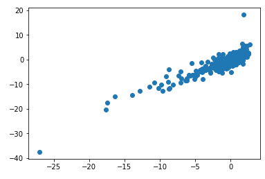
The following scatter plot show Cross Gamma Theta PnL on the x-axis vs the Vega hedged PnL of the risk reversal on y-axis. The regression beta (with 0 intercept) is 1.05 and R^2 is 76%.

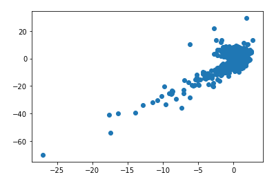
Now I am showing Cross Gamma Theta PnL on x-axis vs total PnL on y-axis. Regression beta is 2.38 and R^2 57%

Answer 1

Great question. Let me try to provide some insights and thoughts regarding the points and questions you raised. It may not be a full answer but hopefully it will help connecting the contents in the paper/book with some trading intuition:

1. From a theoretical perspective, I don't see any mistake in your thinking regarding skew decay but two questions arise from my end: The EuroStoxx backtesting approach in the book (9.10.) is based on the lognormal implied vol dynamic for which Bergomi shows that in the Limit T->0 the skew is constant and independent of ATM vol (that result is actually derived in 8.5.1). Hence, one would suspect that the skew decay component should not really be decisive in his EuroStoxx example, right? I see your valid point though. You say that -based on the skew term structure- this should have a "roll-down" effect in the sense that the skew for 29 should be steeper than for 30d. This brings me to my second question: How exactly did you separate the skew decay P&L in your calculations? It would be nice to have some more detail of your approach. For example, in Figure 9.8. in the book, you can see the impact of different P&Ls to the total P&L of this strategy. What kind of skew decay P&L impact did you get in your approach to the total P&L?

2. You are completely right. The strategy is not peculiar to the restrictions made in the paper/book. The book is approaching this strategy from a very theoretical point of view (short maturity, quadratic vol model etc.). But let's think more practically. The key idea behind this strategy is based on the relationship between Theta and the second derivatives (Gamma, Vanna, Volga), which is also mentioned in the book. You can easily use a break down of Theta into these three components on a maturity slice-by-slice basis and derive implied break even levels for dSpot, dSpot*dVol and dVol. Given the market implied break even levels (which will be different for different slices), you can then evaluate cheapness/richness of these break-even levels based on your own assessment or historical behavior. This is NOT constrained to any of the model restrictions in the book.

Finally, I cannot leave the post without some words of caution. These kind of backtesting strategies are very theoretical and hard (often impossible) to implement in market practice. The following list provides some examples (not limited to!):

• Check the footnotes in the book: "Also, unwinding and restarting a new position on a daily basis is not practical: in our backtest, factoring in a bid/offer spread of 0.2 points of volatility on each leg of our spread position wipes out the strategy’s P&L." But if you don't roll, you quickly get concerned with the next point:

• The strategy may start gamma-neutral but don't ignore the impact of Gamma-speed (third derivatives). In turbulent markets, on the downside you are getting caught short gamma in your delta hedged risk reversal and skew tends to get steeper. A horrible P&L scenario. It may work well if markets are rising (getting you long gamma and skew tends to flatten). So, the strategy -though initially gamma neutral with negligible Volga impact- can quickly turn into a leveraged directional bet. As a hint: Apply your backtesting strategy to data from March 2020 during the peak of the Covid-19 crisis.

• There are more risks involved which may have a significant impact but are not considered in theoretical approaches. For example, what about hedging your delta neutral risk reversal with Futures and the basis between the index and the future explodes to 60 points as there is a high dividend uncertainty in the index?