Geometry of Efficient Frontier of Portfolios

Question

I have been reading about Portfolio Theory, and though the algebra of it seems quite intuitive, I am having a hard time understanding it's geometry.

For the sake of simplicity, I will only talk about two-asset portfolios.

When I came across the term Efficient Frontier for the first time, I wondered why it is shaped that way for any combination of risky assets(Markowitz Bullet). I have not been able to find a concrete answer for that, but I came across a book "Convex Duality and Financial Mathematics" by Carr and Zhu, in which I found a corollary and a note (Pg No.: 39). The corollary relates the mean and the standard deviation of a portfolio by a formula which involves square root. Though I do not understand the corollary, the relation between mean and standard deviation at least gave me a little bit of intuition as to why the Efficient Frontier of two or more risky assets is shaped that way in the mean-standard deviation space. Of course, I would be glad if someone provides a more intuitive idea or reference material about the same.

Then I read that whenever a non-risky asset is in the mix, the Efficient Frontier turns out to be a straight line. In fact, there are three scenarios when the Efficient Frontier would be a straight line, viz.

1. A non-risky asset is involved. The reason, they claim, is that a non-risky asset has no variance and zero correlation with the risky asset. Let A1 be a risky asset and A2 be a non-risky asset, with variances Var_1 and Var_2 respectively. Also, let a1 and a2 be the proportions of the two in the portfolio0. So, the variance of the portfolio, say, Var_p, turns out to be

Var_p = a1^2 . Var_1 + a2^2 . Var_2 + 2.a1.a2.Cov(A1, A2)

  = a1^2 . Var_1   (Since Var_2 = 0 and Cov(A1,A2) = 0)

We may consider expected returns and risk (standard deviation) as parameters (constants) of our model, though that wont be the case in real world. If portfolio variance is to considered as a function of asset weighting, this surely is not a linear relationship, at least in the weighting-risk space.

2. Two perfectly positively correlated risky assets.

Let SD_1 and SD_2 be the standard deviations of the assets.

Here, Var_p = a1^2 . SD_1^2 + a2^2 . SD_2^2 + 2.a1.a2.Cov(A1, A2)

        = a1^2 . SD_1^2 + a2^2 . SD_2^2 + 2.a1.a2.SD_1^2.SD_2^2

        = (a1.SD_1 + a2.SD_2)^2

This, again, is not a linear relationship in the weighting-risk space.

3. Two perfectly negatively correlated assets.

Here, Var_p = (a1.SD_1 - a2.SD_2)^2

Not a linear relationship in the weighting-risk space.

In an effort to understand these relationships, I tried to understand how the expected returns and risks vary w.r.t asset weightings. Since two asset cases are considered here, return and risk can be considered as functions of weight a1 only, since a2 = 1 - a1.

I considered three assets with the following parameters:

1. A1 (Risky) Expected Return = 9.5% Variance = 10%

2. A2 (Risky) Expected Return = 21% Variance = 40%

3. A3 (Non-Risky) Expected Return = 8.5% Variance = 0%

Correlation Coefficients are as follows:

(A1, A2) = 0.05

(A1, A3) = 0

(A2, A3) = 0

I varied the value of a1 from 0 to 1 with an increment of 0.05 to obtain various portfolios.

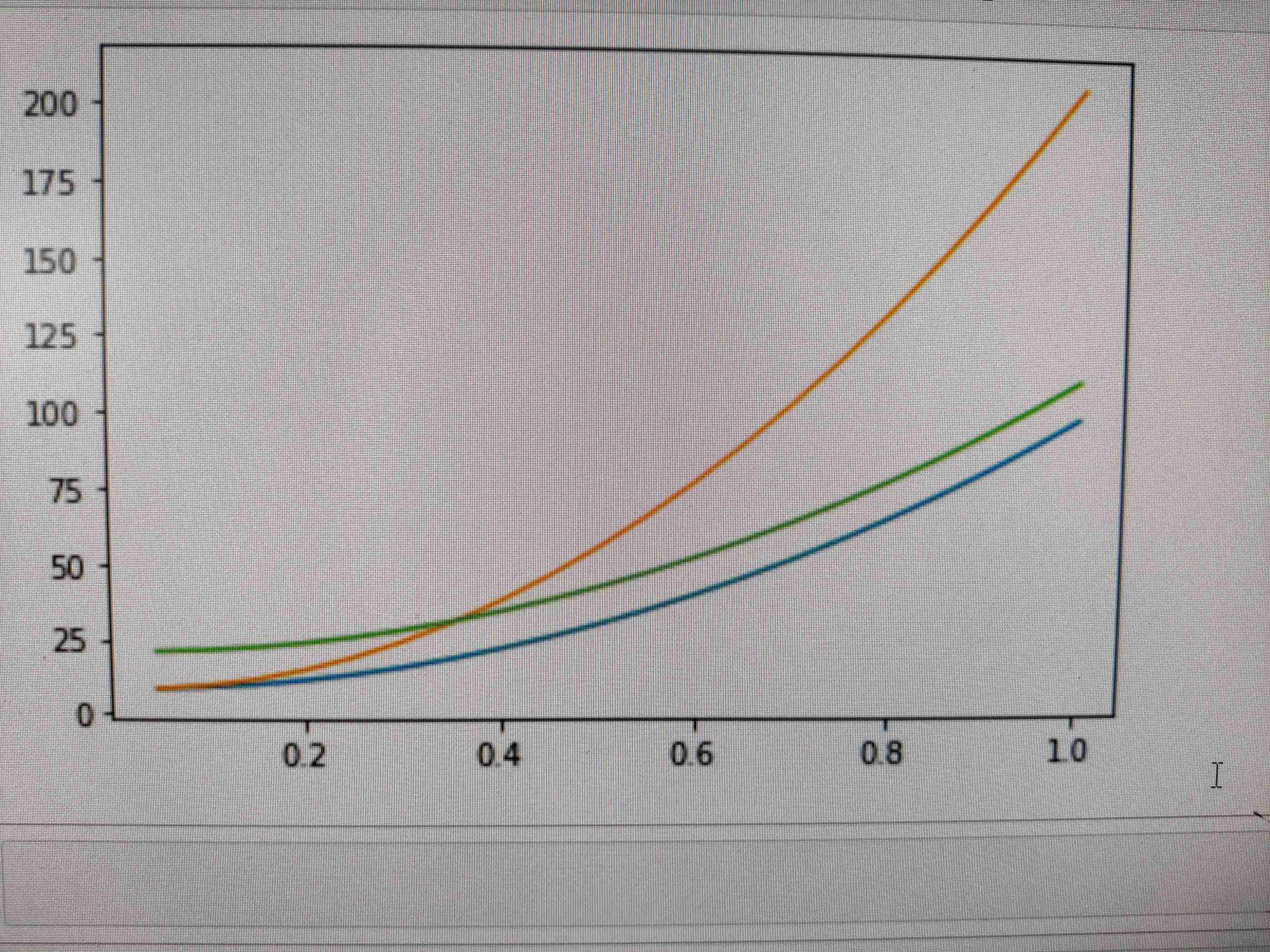
I expected a straight line graph of Expected Returns and weight a1, as the Expected Return of a portfolio is just the weighted average of the returns of the assets. This is just like the equation of a hyperplane. But this is what I got: Blue represents the combination (A1, A3). Green is (A2, A3), and orange is (A1, A2).

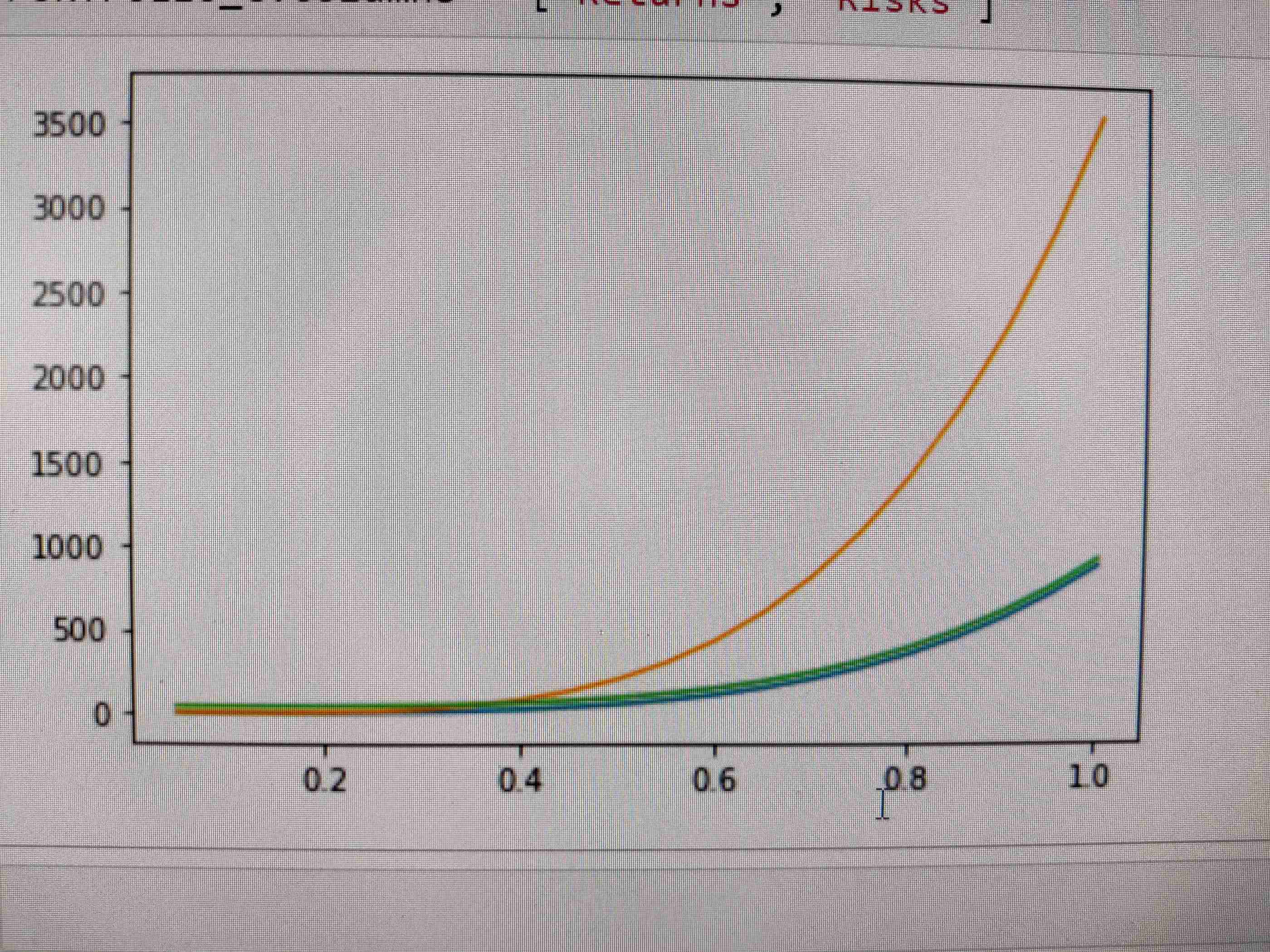
Then I plotted graphs of risk and weight a1, and got this:

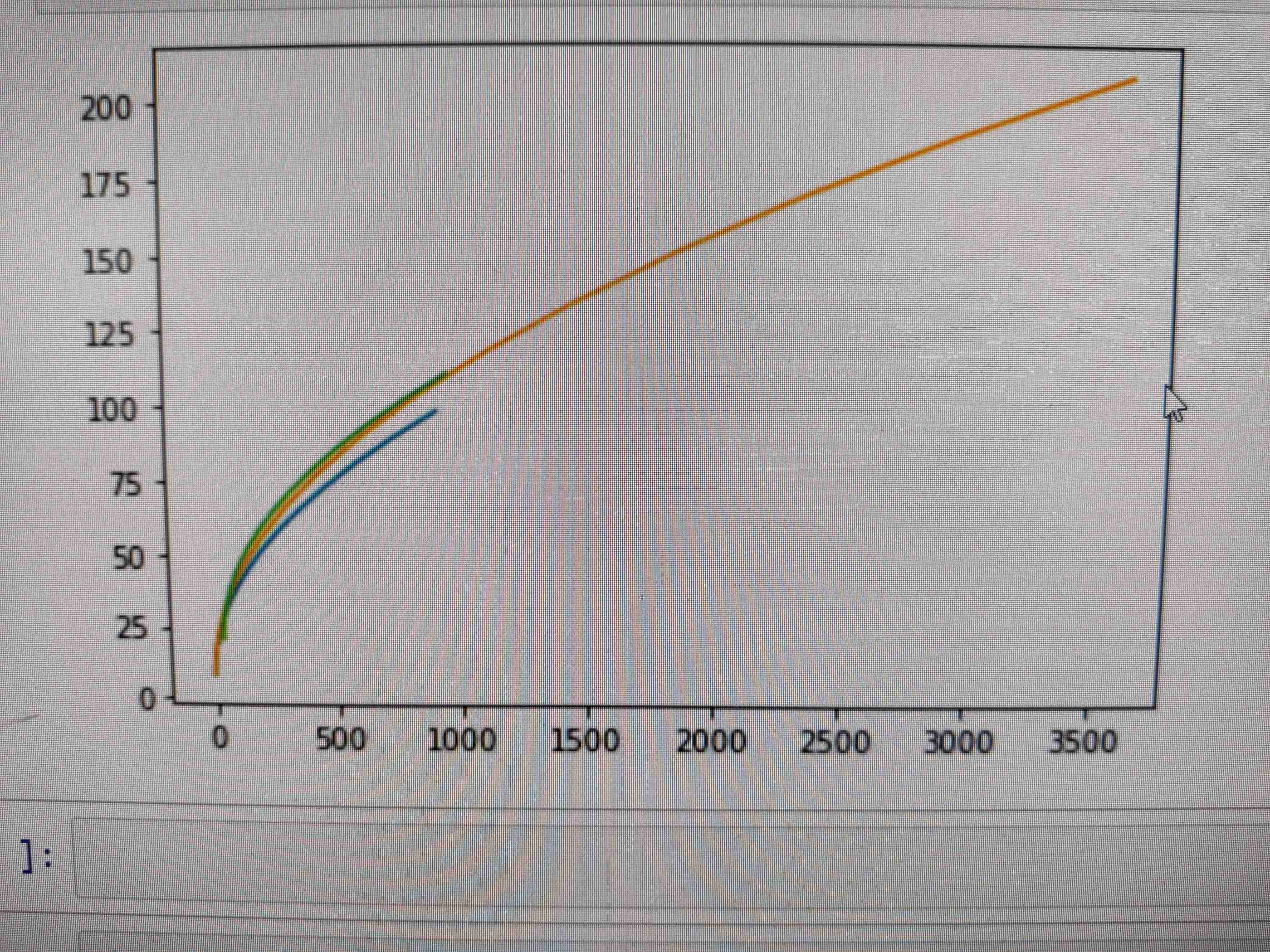
Finally, I plotted the Efficient Frontiers of the three asset combinations, and surprisingly the combinations with a non-risky asset did not generate a straight line Efficient Frontier. See below

So, my questions are as follows:

1. Why the efficient frontiers of risky assets are bullet shaped?

2. Why do we get straight line efficient frontiers when the risk is not related linearly to the asset weights?

3. Why did the simulation show a non linear relationship between portfolio returns and asset weight?

4. Why did the simulation not show straight line efficient frontiers for the risky - non risky combinations?

While questions 3 and 4 might be a result of faulty code; questions 1 and 2, I hope are valid.

Answer 1

Not sure I understand all of your questions. But briefly:

1. If you have a risk free asset, then your efficient portfolios (maximising expected return for given variance) will be on a straight line (when you plot expected return as a function of variance).

2. If you have two assets that are perfectly or perfectly negative correlated, you can construct a risk free portfolio, and are back to 1. Then your variance covariance matrix will be positive semidefinite, instead of positive definite.

3. If you can't construct a risk free portfolio (if your covariance matrix is positive definite), then your efficient portfolios will be on a (sideways) parabola, if you plot their expected return as a function of their variance, and on a hyperbola, if you plot their expected return as a function of their standard deviation. That is probably the bullet you're referring to.