Converting implied volatilities into digital option prices

Question

I have Black and Scholes (1973) implied volatilities computed and I would like to convert these IVs to digital option prices using a Black and Scholes type of formula, I can't find a formula to do this. How can I convert IVs to digital option prices?

Answer 1

In the simplest case, you can just assume a flat vol Black Scholes world. In this case, using the usual BS notation, the fair price of the cash or nothing option is e^(−rt)*N(d2) which is the discounted probability of the option expiring in the money.

Demonstrating this in Julia, you can define this as follows (call price will be needed later).

using Distributions
function BSM(S,K,t,rf,d,σ, cp_flag)
    d1 = ( log(S/K) + (rf - d + 1/2*σ^2)*t ) / (σ*sqrt(t))
    d2 = d1 - σ*sqrt(t)
    value  = cp_flag*exp(-d*t)S*N(cp_flag*d1) - exp(-rf*t)*cp_flag*K*N(cp_flag*d2)
  return value, exp(-r*t)*N(cp_flag*d2)
end

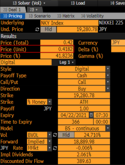
Looking at an example from Bloomberg,

we can compute the following result

# inputs 
s,k , t, σ, r, d  = 19280.78, 19280.78, 1, 0.2471, -0.00006, 0.02061
#result 
res = BSM(s,k,t,log(1+r*t)/t,log(1+d*t)/t,σ, 1)
println("Digital Value per unit = $(round(res[2],digits = 5))")

Bloomberg does not seem to use a call spread in OVME which is why it is so close. Bloomberg does use a call spread in OVML (FX) though. If you were to do this yourself, things get a bit more involved. For example, setting strikes at 𝐾± = 𝐾 ±1/2𝑑𝐾.

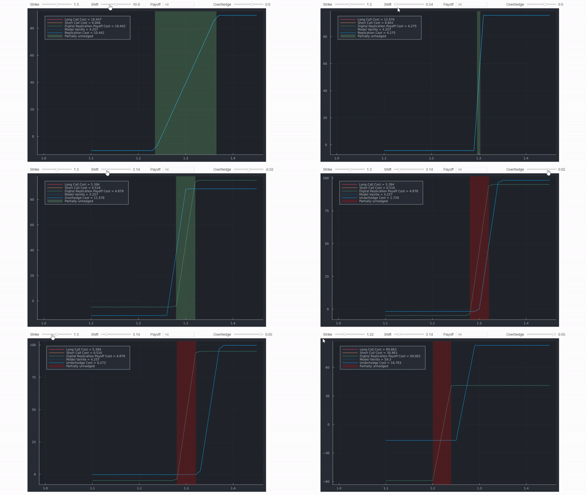
The gif shows this with unrealistic spreads and shifts to make the distinction clear. The actual values however are computed accurately and would match OVML. You can read some details here.

We need to define a few more things to set this up:

• compute the spread (frequently 1% is used, but ideally it is expiry and vol dependent)

function spread(K,shift)
        lower_K = K*(1-shift/2)
        upper_K = K*(1+shift/2)
        spread  = upper_K-lower_K
        return lower_K, upper_K, spread
    end
spr = spread(k,0.01)
val = ("Lower","Upper","Spread")
k = Dict(zip(val,spr))

• Compute the notional adjustment needed to get the desired payoff (The spread * Notional equals the sum of payoffs in the spread scenario - this needs to be adjust to get the desired notional).

    function notional(desiredPayoff,spread)
        scale = desiredPayoff/(spread*desiredPayoff)
        return scale*desiredPayoff
    end

• Fetch the IV for the two strikes (for simplicity I just assume 3 different scenarios: flat, higher vol for lower strike (OTM Put Skew), higher upper strike (OTM Call Skew).

σ = Dict("Lower" =>  [0.2471,0.2473,0.2470], "Upper" =>  [0.2471,0.2470,0.2473] ) 

• compute value (in percent of underlying):

scenario = ["Flat", "OTM Put Skew", "OTM Call Skew"]
res = ["Digital Value per unit ($(scenario[i])) = $((BSM(s,k["Lower"],t, log(1+r*t)/t,log(1+d*t)/t,σ["Lower"][i],1)[1] - BSM(s,k["Upper"],t, log(1+r*t)/t,log(1+d*t)/t,σ["Upper"][i],1)[1])*notional(s,spr[3])/s)" for i in 1:1:3 ]

Answer 2

As pointed out in AKdemy's comment and link, you also need the vanilla IV slope in addition to the level.

Digital put price is $$ \partial_K P(S_t,K) = \partial_K P_{BS}(S_t,K,I(S_t,K)) + \partial_I P_{BS}(S_t,K,I(S_t,K)) \, \partial_K I(S_t,K) $$