added 472 characters in body
Source Link
LocalVolatility
  • 6.1k
  • 4
  • 20
  • 35

Example

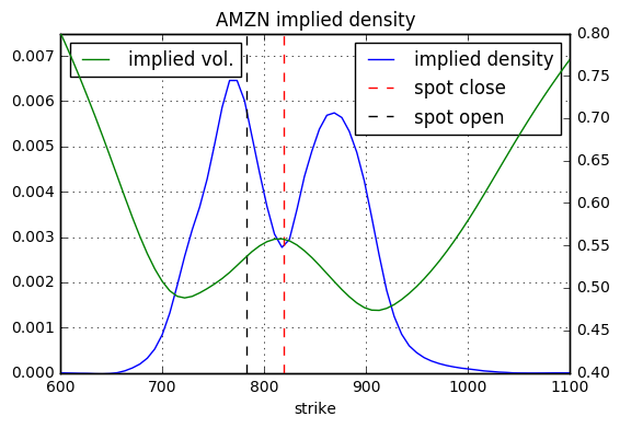
The below image is the implied density of Amazon as of 27th October 2016 for the expiry on 4th November 2016. Amazon was reporting their quarterly earnings after the market close on that day. The implied density was computed using the method in 1). The red dashed line is the closing price pre figures and the black dashed line is the opening price post figures.

enter image description here

References

References

Example

The below image is the implied density of Amazon as of 27th October 2016 for the expiry on 4th November 2016. Amazon was reporting their quarterly earnings after the market close on that day. The implied density was computed using the method in 1). The red dashed line is the closing price pre figures and the black dashed line is the opening price post figures.

enter image description here

References

deleted 14 characters in body
Source Link
LocalVolatility
  • 6.1k
  • 4
  • 20
  • 35

You know that theThe market prices of European plain vanilla calls have to be strictly decreasing and convex in the strike. One approach to fitting them that I like is due to Fengler (2009). He uses cubic smoothing splines and obtains a quadratic program that can be solved very efficiently. Given the piecewise polynomial representation of the option prices, you can easily compute the corresponding densities in closed-form using the usual relationship

However, many common parametrizations wouldn't be able to fit a bi-modal implied probability density. An alternative would be,is to use a polynomial of degree $n$ in the implied volatility along the lines

Finally, you can directly fit the implied distribution. As you mention bi-modal probability densities, I assume you are interested in situations where a jump with a predictable time of occurrence is priced in (e.g. quarterly earning reports). Imagine your "normal" (as in - at all times except for the jump) logarithmic return process followsreturns follow some Levy process $X$, i.e.

Here $p$ is the probability of an up-jump and $\phi(x; \mu, \sigma)$ is the standard normal probability density function. The corresponding characteristic function can be computed in closed-form. Then you use e.g. the Fang and Osterlee (2008) COS method for pricing and calibrate your parameters to the market prices of European plain vanilla options. YouFinally, you can use the same method to compute the implied density of your calibrated model. The beauty of this approach is that you getobtain very easy to interpret parameters.

Yet another possibility to fit the implied probability density directly is by using ana Gram-Charlier series expansion of the normal distribution. The latter is directly parameterized in the higher moments and option prices can be computed very efficiently. A good reference is Schloegel (2013).

You know that the market prices of European plain vanilla calls have to be strictly decreasing and convex in the strike. One approach to fitting them that I like is due to Fengler (2009). He uses cubic smoothing splines and obtains a quadratic program that can be solved very efficiently. Given the piecewise polynomial representation of the option prices, you can easily compute the corresponding densities in closed-form using the usual relationship

However, many common parametrizations wouldn't be able to fit a bi-modal implied probability density. An alternative would be, to use a polynomial of degree $n$ in the implied volatility along the lines

Finally, you directly fit the implied distribution. As you mention bi-modal probability densities, I assume you are interested in situations where a jump with a predictable time of occurrence is priced in (e.g. quarterly earning reports). Imagine your "normal" (as in - at all times except for the jump) logarithmic return process follows some Levy process $X$, i.e.

Here $p$ is the probability of an up-jump and $\phi(x; \mu, \sigma)$ is the standard normal probability density function. The corresponding characteristic function can be computed in closed-form. Then you use e.g. the Fang and Osterlee (2008) COS method for pricing and calibrate your parameters to the market prices of European plain vanilla options. You can use the same method to compute the implied density of your calibrated model. The beauty of this approach is that you get very easy to interpret parameters.

Yet another possibility to fit the implied probability density directly is by using an Gram-Charlier series expansion of the normal distribution. The latter is directly parameterized in the higher moments and option prices can be computed very efficiently. A good reference is Schloegel (2013).

The market prices of European plain vanilla calls have to be strictly decreasing and convex in the strike. One approach to fitting them that I like is due to Fengler (2009). He uses cubic smoothing splines and obtains a quadratic program that can be solved very efficiently. Given the piecewise polynomial representation of the option prices, you can easily compute the corresponding densities in closed-form using the usual relationship

However, many common parametrizations wouldn't be able to fit a bi-modal implied probability density. An alternative is to use a polynomial of degree $n$ in the implied volatility along the lines

Finally, you can directly fit the implied distribution. As you mention bi-modal probability densities, I assume you are interested in situations where a jump with a predictable time of occurrence is priced in (e.g. quarterly earning reports). Imagine your "normal" (as in - at all times except for the jump) logarithmic returns follow some Levy process $X$, i.e.

Here $p$ is the probability of an up-jump and $\phi(x; \mu, \sigma)$ is the standard normal probability density function. The corresponding characteristic function can be computed in closed-form. Then you use e.g. the Fang and Osterlee (2008) COS method for pricing and calibrate your parameters to the market prices of European plain vanilla options. Finally, you can use the same method to compute the implied density of your calibrated model. The beauty of this approach is that you obtain very easy to interpret parameters.

Yet another possibility to fit the implied probability density directly is by using a Gram-Charlier series expansion of the normal distribution. The latter is directly parameterized in the higher moments and option prices can be computed very efficiently. A good reference is Schloegel (2013).

added 6 characters in body
Source Link
LocalVolatility
  • 6.1k
  • 4
  • 20
  • 35

1) FittingModelling the Market Prices

2) FittingModelling the Implied Volatility Smile

3) FittingModelling the Implied Distribution

1) Fitting the Market Prices

2) Fitting the Implied Volatility Smile

3) Fitting the Implied Distribution

1) Modelling the Market Prices

2) Modelling the Implied Volatility Smile

3) Modelling the Implied Distribution

deleted 1 character in body
Source Link
LocalVolatility
  • 6.1k
  • 4
  • 20
  • 35
Loading
Source Link
LocalVolatility
  • 6.1k
  • 4
  • 20
  • 35
Loading