The way that I understand your question is that you are looking to fit the market prices of European plain vanilla options of a single maturity and then back out the corresponding implied probability density function. There are multiple ways that you could approach your problem.
1) Modelling the Market Prices
The market prices of European plain vanilla calls have to be strictly decreasing and convex in the strike. One approach to fitting them that I like is due to Fengler (2009). He uses cubic smoothing splines and obtains a quadratic program that can be solved very efficiently. Given the piecewise polynomial representation of the option prices, you can easily compute the corresponding densities in closed-form using the usual relationship
\begin{equation} e^{r T} \frac{\partial^2 C_0}{\partial K^2}(K) = \mathbb{Q}(K), \end{equation}
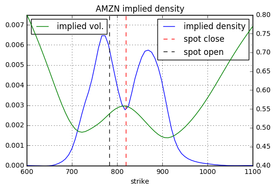
where $\mathbb{Q}(K)$ is the implied probability density function at the strike $K$. Since the fit is very flexible, only ensuring the absence of arbitrage, the resulting density can also be bi-modal.
2) Modelling the Implied Volatility Smile
Alternatively, you could fit a parametric form $\sigma_{\text{IV}}(K)$ to the corresponding implied volatility smile and then use the relationship
\begin{eqnarray} \mathbb{Q}(K) & = & S_0 e^{r T} \phi \left( d_+ \right) \sqrt{T} \left\{ \frac{\partial^2 \sigma_{\text{IV}}}{\partial K^2}(K) + 2 \frac{d_+}{K \sigma_{\text{IV}}(K) \sqrt{T}} \frac{\partial \sigma_{\text{IV}}}{\partial K}(K) \right.\\ & & + \left. \frac{d_+ d_-}{\sigma_{\text{IV}}(K)} \left( \frac{\partial \sigma_{\text{IV}}}{\partial K} \right)^2 + \frac{1}{K^2 \sigma_{\text{IV}}(K) T} \right\}, \end{eqnarray}
see e.g. Fengler (2005) for details.
However, many common parametrizations wouldn't be able to fit a bi-modal implied probability density. An alternative is to use a polynomial of degree $n$ in the implied volatility along the lines
\begin{equation} \sigma_{\text{IV}}(k) = a_0 + a_1 k + a_2 k^2 + \sum_{i = 3}^n \left( a_{i, +} k^i \mathrm{1} \{ k \geq 0 \} + a_{i, -} k^i \mathrm{1} \{ k < 0 \} \right), \end{equation}
where $k = \ln \left( K / F_0(T) \right)$ is the logarithmic moneyness. While this is a flexible parametrization for the near-the-money quotes, you would have to separately deal with the wings. If chosen properly, this has the advantage that i) you can fit very flexible shapes, ii) your calibration problem is linear and iii) you can relatively easily apply the above formula to compute the implied probability density in closed-form. However, it does not ensure that the resulting calibration is free of arbitrage. A very similar approach is to use thin plate splines. It has the same advantages/disadvantages.
If you end up choosing a parametric form for the implied volatility smile that you cannot analytically differentiate, then you could always resort to automatic differentiation libraries. These can help you take exact derivatives (as opposed to finite differences) of almost arbitrary functions.
3) Modelling the Implied Distribution
Finally, you can directly fit the implied distribution. As you mention bi-modal probability densities, I assume you are interested in situations where a jump with a predictable time of occurrence is priced in (e.g. quarterly earning reports). Imagine your "normal" (as in - at all times except for the jump) logarithmic returns follow some Levy process $X$, i.e.
\begin{equation} \ln \left( S_t / S_0 \right) = \gamma t + X_t, \end{equation}
where $\gamma$ is some drift term (that you need to chose such that the stock price becomes a martingale). You can then augment these dynamics by a single predictable jump $Y$
\begin{equation} \ln \left( S_t / S_0 \right) = \gamma t + X_t + Y \mathrm{1} \left\{ t \geq t_J \right\} \end{equation}
where $Y$ follows e.g. a Gaussian mixture with probability density function
\begin{equation} f_Y(X) = p \phi \left( x; \mu_+, \sigma_+ \right) + (1 - p) \phi \left( x; \mu_-; \sigma_- \right). \end{equation}
Here $p$ is the probability of an up-jump and $\phi(x; \mu, \sigma)$ is the standard normal probability density function. The corresponding characteristic function can be computed in closed-form. Then you use e.g. the Fang and Osterlee (2008) COS method for pricing and calibrate your parameters to the market prices of European plain vanilla options. Finally, you can use the same method to compute the implied density of your calibrated model. The beauty of this approach is that you obtain very easy to interpret parameters.
Yet another possibility to fit the implied probability density directly is by using a Gram-Charlier series expansion of the normal distribution. The latter is directly parameterized in the higher moments and option prices can be computed very efficiently. A good reference is Schloegel (2013).
Example
The below image is the implied density of Amazon as of 27th October 2016 for the expiry on 4th November 2016. Amazon was reporting their quarterly earnings after the market close on that day. The implied density was computed using the method in 1). The red dashed line is the closing price pre figures and the black dashed line is the opening price post figures.
References
Fang, Fang and Cornelis W. Oosterlee (2008) "A Novel Pricing Method for European Options Based on Fourier-Cosine Series Expansions", Siam Journal of Scientific Computing, Vol. 31, No. 2, pp. 826-848
Fengler, Matthias R. (2005) "Semiparametric Modeling of Implied Volatility", Springer Finance
Fengler, Matthias R. (2009) "Arbitrage-Free Smoothing of the Implied Volatility Surface", Quantitative Finance, Vol. 9, No. 4, pp. 417-428
Schloegel, Erik (2013) "Option Pricing Where the Underlying Assets Follow a Gram/Charlier Density of Arbitrary Order", Journal of Economic Dynamics and Control, Vol. 37, No. 3, pp. 611-632

