I'm trying to simulate a process as close as possible to EUR/USD of the ten past years.
I've used a Ornstein-Uhlenbeck process:
$$d X_t = -\theta (X_t - \mu) d t + \sigma d B_t$$
with the parameters $\mu$, $X_0$, $\theta$, $\sigma$ being calibrated such that mean, standard deviation, total absolute variation (i.e. $\sum_i |X_{t_{i+1}} - X_{t_i}|$ for a given sampling rate) are as close as possible to the real historical data. For example I used $\mu \approx$ 1.3 $ / 1 €.
The only thing that fails is that the created process doesn't have big spikes whereas the real historical data sometimes shows such jumps.
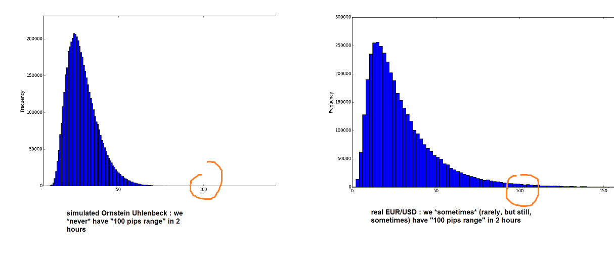
More precisely, here is the histogram of the range over 2 hours (each $X_t$ represents one minute, so 120 means 2 hours): $$range_t = \max_{k \leq 120} X_{t-k} - \min_{k \leq 120} X_{t-k}$$
Question:
The simulated O-U process I did is too "nice and gentle": the range in 2 hours never exceeds 100 pips, whereas in real-life, the range in 2 hours can exceed 100 pips. How to make it more like the real data?
How should I improve the model (i.e. the Stochastic Differential Equation) to have more "big ranges"? Add some "jump diffusion" (with which method)? Make $\sigma$ vary, and how?
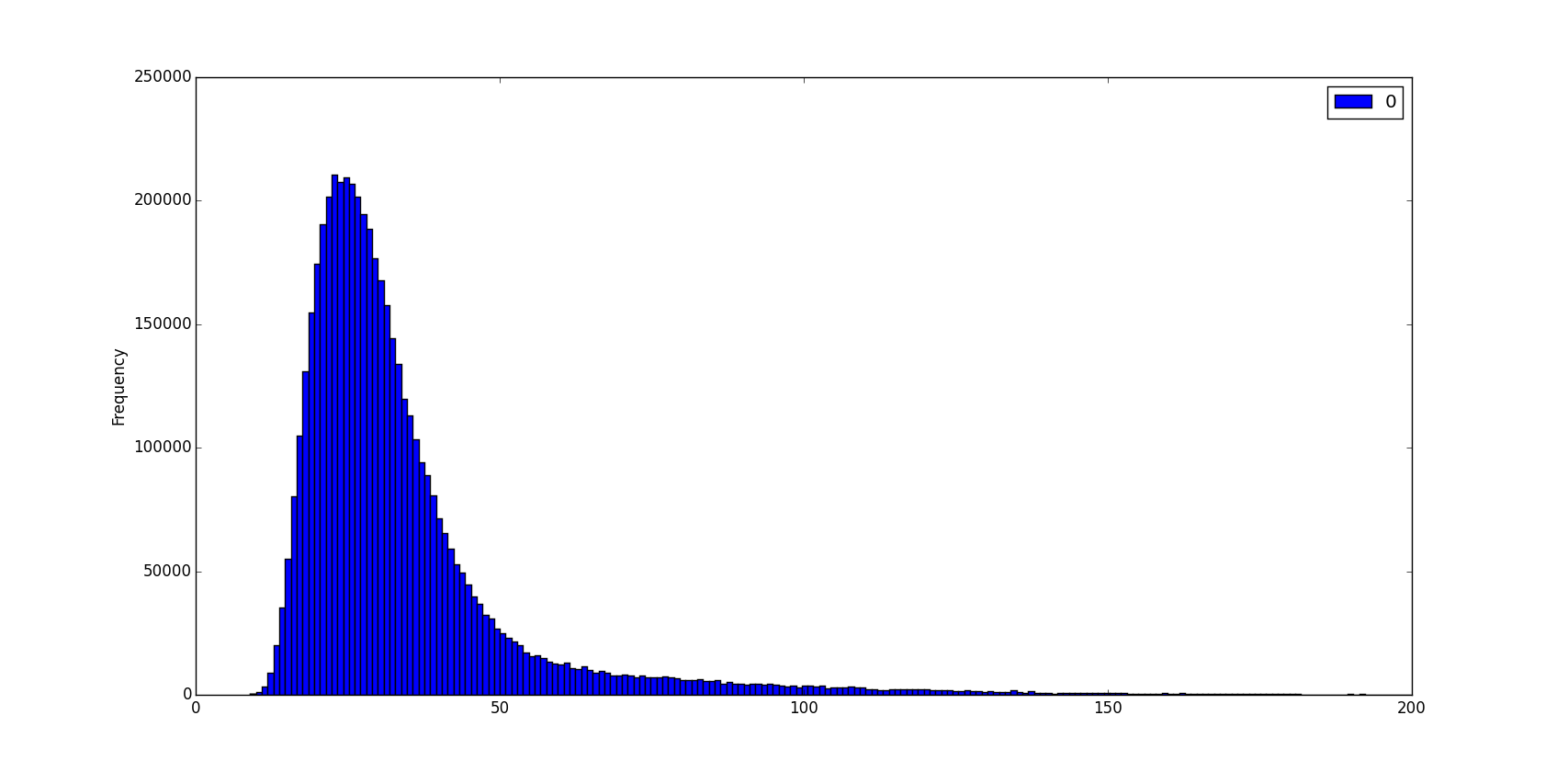
EDIT: I tried to add a "jump" term $d\, q_t$ to the SDE, i.e. very rarely we have a "jump" of height $h$ pips, with $h \sim \pm 0.0060 \cdot Log\mathcal{N}(0,1)$, i.e. a "jump" of average height 60 pips (with random sign + or -).
This has an effect of having a heavier tail for the "2hours range" distribution:
but even by choosing the right parameters, the "heavier tail" still doesn't look like the real EURUSD "2 hours range" histogram tail...
Another option: Should I replace $d\, B_t$, which is a $\mathcal{N}(0, \sigma)$ by another random variable with a higher kurtosis? Which one?


