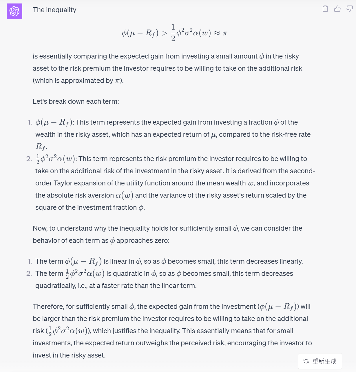
The following question is from Kerry E. Back's textbook, and I struggle with it many days, but I wonder this question could be trivial for expertises. If anyone can help, I will really apreciate it!
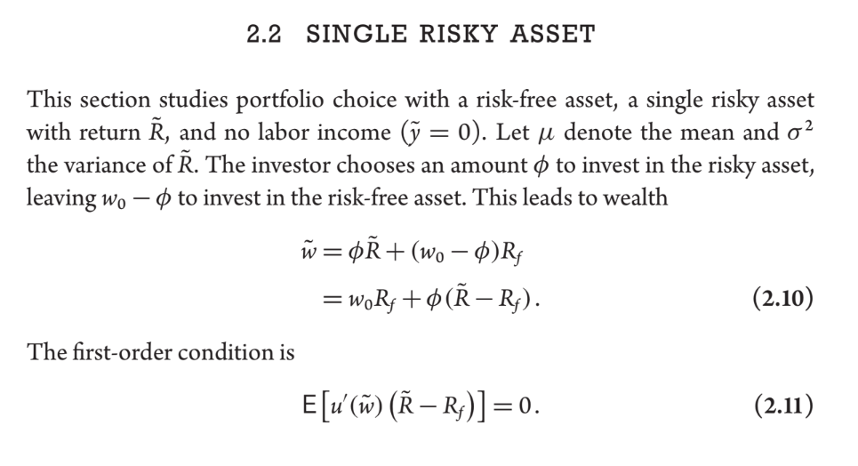
Given the first order condition (2.11) of the portfolio optimiztion problem with single risky asset: $\mathrm{E}\left[u^{\prime}(\tilde{w})\left(\tilde{R}-R_f\right)\right]=0$. The textbook says that:
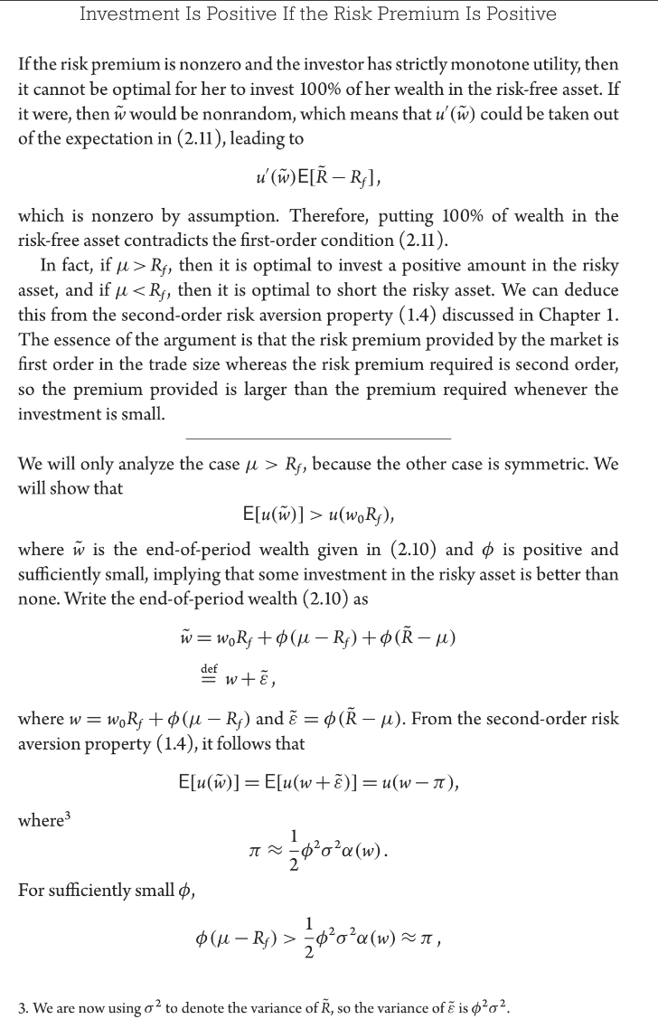
If the risk premium is nonzero and the investor has strictly monotone utility, then it cannot be optimal for her to invest $100 \%$ of her wealth in the risk-free asset. If it were, then $\tilde{w}$ would be nonrandom, which means that $u^{\prime}(\tilde{w})$ could be taken out of the expectation in (2.11), leading to $$ u^{\prime}(\tilde{w}) \mathrm{E}\left[\tilde{R}-R_f\right], $$ which is nonzero by assumption. Therefore, putting $100 \%$ of wealth in the risk-free asset contradicts the first-order condition (2.11).
In fact, if $\mu>R_f$, then it is optimal to invest a positive amount in the risky asset, and if $\mu<R_f$, then it is optimal to short the risky asset. We can deduce this from the second-order risk aversion property (1.4) discussed in Chapter 1. The essence of the argument is that the risk premium provided by the market is first order in the trade size whereas the risk premium required is second order, so the premium provided is larger than the premium required whenever the investment is small.
I don't have any question about this part, but the footnote mentions that:
We will only analyze the case $\mu>R_f$, because the other case is symmetric. We will show that $$ \mathrm{E}[u(\tilde{w})]>u\left(w_0 R_f\right), $$ where $\tilde{w}$ is the end-of-period wealth given in (2.10) and $\phi$ is positive and sufficiently small, implying that some investment in the risky asset is better than none. Write the end-of-period wealth (2.10) as $$ \begin{aligned} \tilde{w} & =w_0 R_f+\phi\left(\mu-R_f\right)+\phi(\tilde{R}-\mu) \\ & \stackrel{\text { def }}{=} w+\tilde{\varepsilon}, \end{aligned} $$ where $w=w_0 R_f+\phi\left(\mu-R_f\right)$ and $\tilde{\varepsilon}=\phi(\tilde{R}-\mu)$. From the second-order risk aversion property (1.4), it follows that $$ \mathrm{E}[u(\tilde{w})]=\mathrm{E}[u(w+\tilde{\varepsilon})]=u(w-\pi), $$ where $$ \pi \approx \frac{1}{2} \phi^2 \sigma^2 \alpha(w) $$ For sufficiently small $\phi$, $$ \phi\left(\mu-R_f\right)>\frac{1}{2} \phi^2 \sigma^2 \alpha(w) \approx \pi $$ Note 1:$\phi$ is the amount of risky asset that chosen by investor.
Note 2:We are now using $\sigma^2$ to denote the variance of $\tilde{R} $, so the variance of $\tilde{\varepsilon}$ is $\phi^2 \sigma^2$.
Note 3:$\tilde{R}$ is the return of the risky asset, $R_f$ is the return of the risk-free asset$.\mu$ denotes the mean and $\sigma^2$ the variance of $\tilde{R}$.
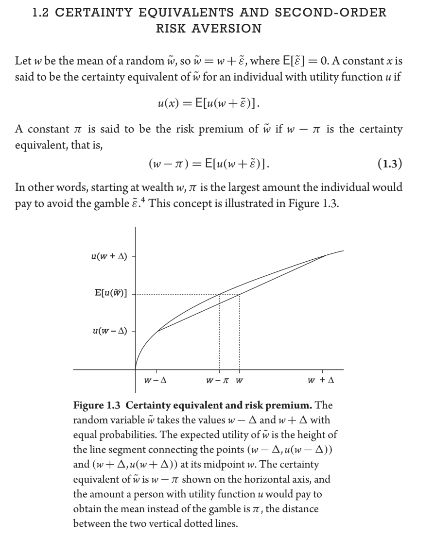
Note 3.5:$\alpha(w)$ is the absolute risk aversion. $\pi$ is the risk premium of random $\tilde{w}$. $w$ be the mean of a random $\tilde{w}$ , so $\tilde{w}=w+\tilde{\varepsilon}$, where $\mathrm{E}[\tilde{\varepsilon}]=0$.
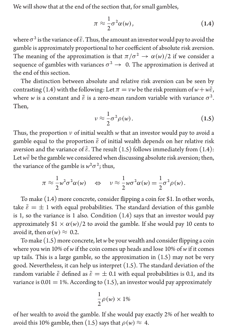
Note 4:The property (1.4) says that for small gambles, $$ \pi \approx \frac{1}{2} \sigma^2 \alpha(w), $$ where $\sigma^2$ is the variance of $\tilde{\varepsilon}$ (In chapter 1, not in this case. For this case, see Note 2.). Thus, the amount an investor would pay to avoid the gamble is approximately proportional to her coefficient of absolute risk aversion. The meaning of the approximation is that $\pi / \sigma^2 \rightarrow \alpha(w) / 2$ if we consider a sequence of gambles with variances $\sigma^2 \rightarrow 0$.
My question is: Why the final inequality holds for sufficiently small $\phi$?
Here are some captures from the textbook that related to my question:

