5
$\begingroup$

I am seeing an issue when callibrating an MP distribution. Assume a log return series for the SP500 with the following dimensions

dim(xts.sp500.ret.stocksonly)

==> [1] 1133 478

sp500.cor <- cor.empirical(xts.sp500.ret.stocksonly)
sp500.eigens <- eigen(sp500.cor)$values
sp500.eigen.density <-  density(sp500.eigens,n=5000)
plot(sp500.eigen.density,xlim=c(0,4),main="sp500 returns eigenvalue density")

I assume my 'Q' value is 1133/478 =
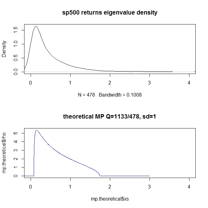
eigenvalues sp500

Problem: Even though the 'shape' and cutoffs seem OK -- the density value (y axis) seem vastly OFF. Peak of 1.5 for the real series - 5 or so for the theoretical, (note I am truncating the plot so the market eigenvalues are not shown, they are huge around 200).

Question: 1) Is this expected? 2) How does this affect callibration? Should I trust the results and simply look at the cutoffs? 3) Also when 'cleansing' the matrix I see most code (e.g. filter.RMT in tawny) simply replaces values below Lambda+ with the average, what about Lambda- though?

thanks much!

$\endgroup$
1
  • $\begingroup$ What is an MP distribution? $\endgroup$ Commented Feb 12, 2021 at 16:28

1 Answer 1

2
$\begingroup$
  1. The plot function is smoothing the plot. You should show the distribution of eigenvalues via a bar chart. Because a bar chart is discrete you can better discern the separation of the top-most eigenvaules. The top-most eigenvalue (representing the market factor) should be substantially greater than bulk of the eigenvalue distribution.

  2. I assume by "calibration" you mean "eigenvalue cleansing". The approach would be to apply the RMT cleansing procedure on eigenvalues beneath the upper noise-band (lambda+)

  3. The procedure of replacing eigenvalues below Lambda+ with the average will by definition also replace values below Lambda- as well. Replacing the eigenvalues by the average is one of many possible cleansing procedures.

$\endgroup$
2
  • $\begingroup$ Clarification to the question: By callibration I mean how to fit the correct MP distribution to the eigenvalues density I get. Notice in the top plot the max "y" value I get is ~1.5, while for the MP distribution from theory the values are much higher. How do I know i've made a good fit of the MP parameters? thanks. $\endgroup$ Commented Jan 21, 2012 at 23:29
  • $\begingroup$ The empirical distribution of eigenvalues does not match the MP distribution because the former contains non-random factors. The theory shows what the eigenvalue distribution is for a random symmetric matrix for some choice of Q and Sigma. You can calculate Q and Sigma directly using the asymptotic definition of Q (which you have in your post), and sigma is simply the sigma of the elements of the de-meaned symmetric covariance matrix. So there is no need to "fit" the empirical distribution. $\endgroup$ Commented Jan 22, 2012 at 1:47

Your Answer

By clicking “Post Your Answer”, you agree to our terms of service and acknowledge you have read our privacy policy.

Not the answer you're looking for? Browse other questions tagged or ask your own question.