Is it possible to approach finding the risk premium of this derivative using Ito's Lemma?

Question

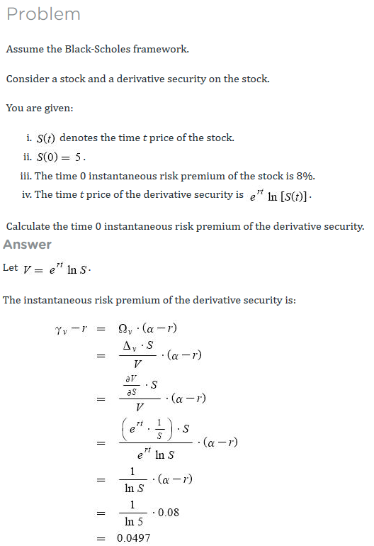
I understand the author's intended solution to the below problem, but I thought I would see if I could solve this using first principles and Ito's Lemma instead for practice.

Let $V(S(t), t) = e^{rt}\ln{[S(t)]}$. Then

\begin{align*}V_S &= \frac{e^{rt}}{S(t)},\\ V_{SS} &= \frac{-e^{rt}}{[S(t)]^2} \text{, and}\\ V_t &= re^{rt}\ln[S(t)].\end{align*}

Assuming the Black-Scholes framework, $dS(t) = (\alpha - \delta)S(t) dt + \sigma S(t) dZ(t)$. By Ito's Lemma,

\begin{align*}dV &= (\alpha - \delta)e^{rt} dt +e^{rt}\sigma dZ(t) - \frac{1}{2}e^{rt}\sigma^2 dt + re^{rt}\ln[S(t)]dt\\ &=[(\alpha - \delta)e^{rt} - 0.5e^{rt}\sigma^2 + re^{rt}\ln[S(t)]dt + e^{rt}\sigma dZ(t).\end{align*}

It would appear that without knowing anything about $\delta$ or $\sigma$, we have no where to go. So is there not a way to solve this problem from first principles without knowing that since the Sharpe ratios of the asset and the derivative are perfectly (positively) correlated, they are equal? I.e.,

$$\frac{\gamma_V - r}{\sigma_V} = \frac{\gamma - r}{\Omega_V\sigma} = \frac{\alpha - r}{\sigma},$$

where $\gamma_V$ is the continuously compounded return on the derivative and $\Omega_V$ is the elasticity of the derivative.

Answer 1

Assume that under the real world measure $$ dS_t/S_t = (\alpha-\delta) dt + \sigma dZ_t^\Bbb{P} \tag{1} $$ Under the EMM $\Bbb{Q}$ one then needs to have (fundamental theorem of asset pricing: in the absence of arbitrage the discounted value of any self-financing portfolio should be a martingale): $$ dS_t/S_t = (r-\delta) dt + \sigma dZ_t^\Bbb{Q} \tag{2} $$ Examining $(1)$ and $(2)$ the (instantaneous) excess return per unit of volatility risk is therefore: $$ \pi_S = \frac{\alpha-\delta}{\sigma} - \frac{r-\delta}{\sigma} := \frac{\alpha-r}{\sigma} $$

---

Now assume $V(t,S_t) = e^{rt} \ln(S_t)$. As you noted, applying Itô's lemma yields: $$ dV_t = e^{rt}\left[ r\ln(S_t) dt + \frac{dS_t}{S_t} - \frac{1}{2} \sigma^2 dt \right] \tag{3} $$ Writing $dV_t$ under real world and risk-neutral measures respectively plugging $(1)$ and $(2)$ then gives: $$ dV_t = e^{rt}\left[ (\alpha-\delta) + r\ln(S_t) - \frac{1}{2} \sigma^2 \right] dt + e^{rt} \sigma dZ_t^\Bbb{P} \tag{4} $$ $$ dV_t = e^{rt}\left[ (r-\delta) + r\ln(S_t) - \frac{1}{2} \sigma^2 \right] dt + e^{rt} \sigma dZ_t^\Bbb{Q} \tag{5} $$ The (instantaneous) excess return per unit of volatility risk is now: $$ \pi_V = \frac{e^{rt}\left((\alpha-\delta) + r\ln(S_t) - \frac{1}{2} \sigma^2 \right)}{e^{rt}\sigma} - \frac{e^{rt}\left( (r-\delta) + r\ln(S_t) - \frac{1}{2} \sigma^2 \right)}{e^{rt}\sigma} := \frac{\alpha-r}{\sigma} = \pi_S $$ So you see that you fall back on the result that the Sharpe ratios are the same without any prior knowledge.