3
$\begingroup$

I am trying to model the future prices of a number of commodities. For this, I am applying geometric Brownian motion, writing a Monte Carlo code in Python. Given that I want to estimate tommorows price $S_t$ of a commodity, I am using the equation:

$S_{t}=S_{t-1}\exp((\mu-\frac{\sigma^2}{2})+z\sigma)$

Where $z$ is determined from a stochastic number from a normal distribution. $\sigma$ and $\mu$ I have calculated using the log-"returns" based on annual price data from the respective commodity, i.e. from $t_0$ to $t$. The data I have is between 1950-2015.

Now, I want to model future prices until 2050, counting from 2015. So I have applied the aforementioned formula for each year, starting from 2015 until 2050. For instance, the price year 2041 would be:

$S_{2041}=S_{2040}\exp((\mu-\frac{\sigma^2}{2})+z\sigma)$

I have performed 1000 simulations, obtaining a wide range for the price in 2050. I understand this method is not appropiate for forecasting, but what can I do with my results to say something about the future price? If I take the mean of my results, and I run many simulations, it is equivalent to just apply the formula $S_t=S_{t-1}\exp(\mu*\Delta t)$, right? I cannot assume that this mean is a good forecast estimate, or can I?

Assume that I will buy this commodity in 2050, and there is a risk that the real price will increase, how can I apply this Monte Carlo simulation model to determine how much money I need to save in order to afford the commodity in 2050? I think that it is something like a risk calculation that I am looking for.

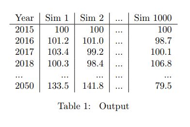
Simulation results

$\endgroup$

2 Answers 2

1
$\begingroup$

The future price has a lognormal distribution, so its moments can be calculated exactly using the fitted parameter values (or looked up). Confidence intervals for parameter estimates will give c.i. for moments of future prices too.

$\endgroup$
1
  • $\begingroup$ Thank you for the answer. I have edited my question, and you can now see my results. So as you commented, each column would be lognormally distributed. But I do not quite understand what you mean with "its moments can be calculated exactly using the fitted parameter values". I have calculated the 95%-CI for each row (year). What I have done so far, is to calculate the mean for each row, i.e. the mean of all simulations for each year. But how should I interpret this? Plotting it just gives me a exponential curve. $\endgroup$
    – Andr
    Commented Jun 26, 2018 at 13:18
0
$\begingroup$

You are right, the mean is going to be $S_0 e^{\mu t}$. You may want to increase the number of simulations by the way, 1,000 ain’t that many. Since you know $(S_t)$ analytically in closed form, simulating and averaging does not really provide you with any further information. We know all moments of $(S_t)$ in closed-form anyway and can compute probabilities of all events analytically (e.g. how likely is it that $S_t$ is greater than $x$ for a certain $t$). Note that one typically uses approximations (simulations) if one does not have have analytical formulae. So, you can you interpret your results? All you can do is to 'numerically verify' that you arrive at the same values as the closed formula as you increase the number of simulations.

You can’t really use this method to forecast prices though. Asset prices almost certainly do not follow a geometric Brownian motion, so your results are going to be far off from the real world. You would need a more realistic model.

$\endgroup$

Your Answer

By clicking “Post Your Answer”, you agree to our terms of service and acknowledge you have read our privacy policy.

Not the answer you're looking for? Browse other questions tagged or ask your own question.