How to perform Monte Carlo simulations to price a Forward contract under the Schwartz mean reverting model?

Question

Objective: (1) Implement the Euler Explicit Method for solving the PDE for option prices under the Schwartz mean reverting model. (2) Compare with a Monte Carlo simulation.

I'm stuck with point 1 (see this question) so in the meanwhile I'm working on point 2. Basically, I have 200 monthly spot prices of a commodity (oil) following the Schwartz mean reverting SDE $dS = \alpha(\mu-\log S)Sdt + \sigma S dW$. This commodity is the underlying asset of the Forward contract with price at delivery $F(S,T)$, where $S$ is the spot price at time 0 and $T$ is the expiry time. Such a contract is equivalent to having an option with $\text{payoff}(S_T)=S_T-K$, where $K=F(S,T)$ is the strike price.

Letting $\tau=T-t$ be the time to expiry, the formula for the price of the forward contract is

$$\tag{1}F(S,\tau)=\exp\Big(e^{-\alpha\tau}\log S +(\mu-\frac{\sigma^2}{2\alpha}-\frac{\mu-r}{\alpha})(1-e^{-\alpha\tau})+\frac{\sigma^2}{4\alpha}(1-e^{-2\alpha\tau})\Big)$$

and the value of the equivalent option is $V(S,t)=e^{-r(T-t)}F(S,t)$. ($\alpha, \sigma, \mu$ are estimated from data)

Knowing this information, how to run (I'm using matlab but other languages are fine too) a Monte Carlo simulation to price the option?

I read these are the steps

• generate a large number of random price paths for the underlying asset
• for each path compute the payoff of the option
• compute the average of all payoffs
• discount the average to today

but since I'm working with real data of oil spot prices, I'm a bit confused: how can we obtain the value of the option having an underlying commodity with known spot prices by generating random spot price paths?

Moreover how to perform the next steps using the above formulas?

---

EDIT: First attempt

I wrote the code which computes what I think (can you confirm?) is the exact solution for option pricing (V_exact) and then computes the approximating solution by means of Monte Carlo simulation (V_Monte_Carlo). The MC simulation uses the first spot price (real data) and the estimated parameters to 'randomly' compute the next spot prices. To compute the spot prices, instead of using the equation for $dS$ that I wrote above it's easier to use this one which is obtained from $dS$ by letting $X=\log S$.

$$\tag{2}X_t = X_0 e^{-\alpha t} + \mu^*(1-e^{-\alpha t}) + \underbrace{\sigma e^{-\alpha t} \int_0^t e^{\alpha s} dW_s}_Z$$

where $\mu^* = \mu-\dfrac{\sigma^2}{2\alpha}$ and $Z \sim \sigma\sqrt{\dfrac{1-e^{-2\alpha t}}{2\alpha}} \cdot N(0,1)$

These are the steps for the Monte Carlo simulation:

1. The first price F of the forward contract - and so of the option V too - is set to 0 since there is no cost to enter a forward contract. Compute the first value of $X$ by taking the logarithm of the first spot price
2. compute the next value of $X$ using the formula (2)
3. compute the next value of the spot price by taking the exponential of $X$
4. compute the next price F of the forward contract using formula (1)
5. compute the next price V of the option using $V(S,t)=e^{-r(T-t)}F(S,t)$
6. compute the average V_Monte_Carlo of the option prices
7. repeat steps 2-6 until all values are computed

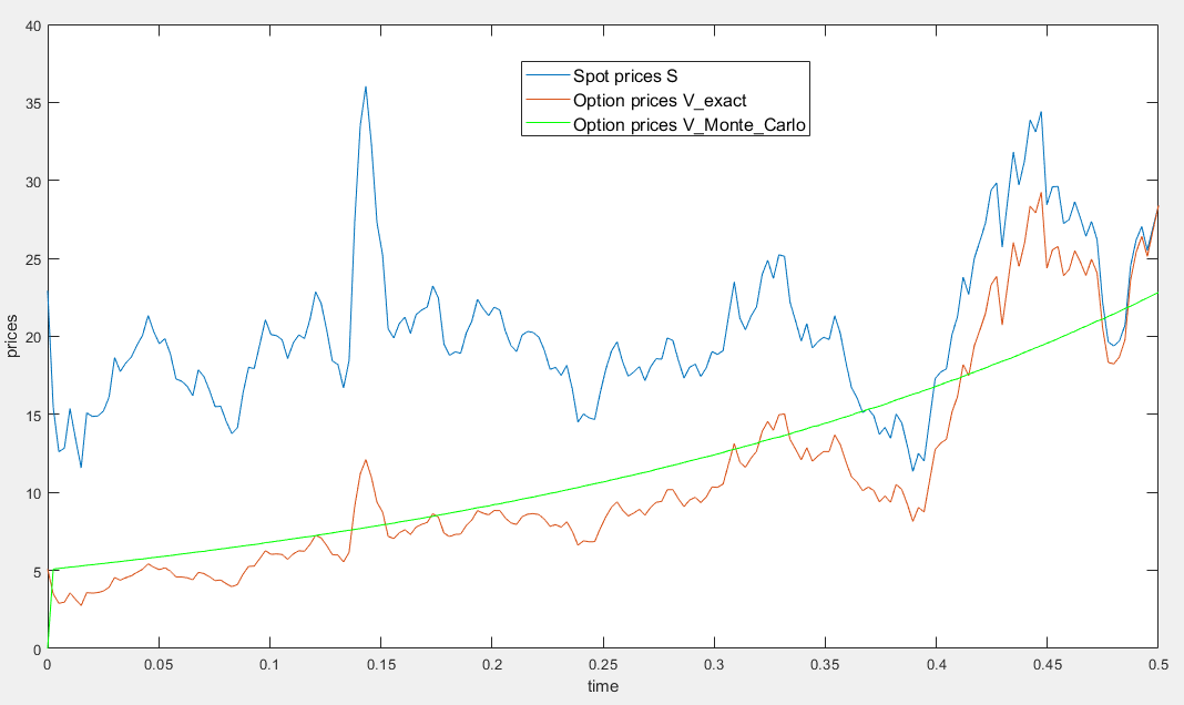
However, as you can see from the image below, the curve of the option prices obtained with the MC simulation is smooth, while what I was expecting was a curve similar to the one of the exact solution. So I made some mistakes somewhere

% S = oil spot prices
S = [ 22.93 15.45 12.61 12.84 15.38 13.43 11.58 15.10 14.87 14.90 15.22 16.11 18.65 17.75 18.30 18.68 19.44 20.07 21.34 20.31 19.53 19.86 18.85 17.27 17.13 16.80 16.20 17.86 17.42 16.53 15.50 15.52 14.54 13.77 14.14 16.38 18.02 17.94 19.48 21.07 20.12 20.05 19.78 18.58 19.59 20.10 19.86 21.10 22.86 22.11 20.39 18.43 18.20 16.70 18.45 27.31 33.51 36.04 32.33 27.28 25.23 20.48 19.90 20.83 21.23 20.19 21.40 21.69 21.89 23.23 22.46 19.50 18.79 19.01 18.92 20.23 20.98 22.38 21.78 21.34 21.88 21.69 20.34 19.41 19.03 20.09 20.32 20.25 19.95 19.09 17.89 18.01 17.50 18.15 16.61 14.51 15.03 14.78 14.68 16.42 17.89 19.06 19.65 18.38 17.45 17.72 18.07 17.16 18.04 18.57 18.54 19.90 19.74 18.45 17.33 18.02 18.23 17.43 17.99 19.03 18.85 19.09 21.33 23.50 21.17 20.42 21.30 21.90 23.97 24.88 23.71 25.23 25.13 22.18 20.97 19.70 20.82 19.26 19.66 19.95 19.80 21.33 20.19 18.33 16.72 16.06 15.12 15.35 14.91 13.72 14.17 13.47 15.03 14.46 13.00 11.35 12.51 12.01 14.68 17.31 17.72 17.92 20.10 21.28 23.80 22.69 25.00 26.10 27.26 29.37 29.84 25.72 28.79 31.82 29.70 31.26 33.88 33.11 34.42 28.44 29.59 29.61 27.24 27.49 28.63 27.60 26.42 27.37 26.20 22.17 19.64 19.39 19.71 20.72 24.53 26.18 27.04 25.52 26.97 28.39 ];
r = .1;    % yearly instantaneous interest rate
T = 1/2;   % expiry time

alpha = 0.0692;
sigma = 0.0876; % values estimated from data
mu = 3.0582;

t = linspace(0,T,numel(S));
tau = T-t;
lambdahat = (mu-r)/alpha;
muhat = mu-sigma^2/2/alpha-lambdahat;

%% Is this V the exact solution?
% this F is the formula (1) on stackexchange
F = exp( exp(-alpha*tau).*log(S) + muhat*(1-exp(-alpha*tau)) + sigma^2/4/alpha*(1-exp(-2*alpha*tau)) );
% K = F(end); % shouldn't we use also the strike price?
V_exact = exp( -r*tau ) .* F; % V contains the prices of the option
plot(t,S)
hold on
plot(t,V_exact)

%% Monte Carlo simulation
n = numel(S);
N = 10000; % number of samples
mustar = mu-sigma^2/2/alpha;
X = zeros(N,n);
X(:,1) = log(S(1));
S = zeros(N,n);
S(:,1) = S(1);
F = zeros(N,n);
V = zeros(N,n);
V_Monte_Carlo = zeros(1,n);
dt = 1; % which values for dt has to be pick?
for k = 2:n
    tau = T-t(k);
    % this X is the formula (2) on stackexchange
    X(:,k) = X(k-1)*exp(-alpha*dt) + mustar*(1-exp(-alpha*dt)) + sigma*sqrt(1-exp(-2*alpha*dt))/sqrt(2*alpha)*randn(N,1);
    S(:,k) = exp(X(:,k));
    F(:,k) = exp( exp(-alpha*tau).*log(S(:,k)) + muhat*(1-exp(-alpha*tau)) + sigma^2/4/alpha*(1-exp(-2*alpha*tau)) );
    V(:,k) = exp(-r*tau)*F(:,k);
    V_Monte_Carlo(k) = mean(V(:,k));
end
plot(t,V_Monte_Carlo,'g')
legend('Spot prices (S)','Option prices (V) from exact solution','Option prices from Monte-Carlo simulation')

Answer 1

Let's see.

You have the following SDE for the stock price under the measure $P$:

$$ dS(t) = \alpha \cdot (\mu - \log S(t)) \cdot S(t) \cdot dt + \sigma \cdot S \cdot dW^P(t), $$

with initial condition $S(0) = S_0$. Moreover, defining $X(t) = \log S(t)$, assuming a constant market price of risk $\lambda = \mu - r$ and performing a change of measure, you get the process $X(t)$ under the risk neutral measure $Q$ as:

$$ dX(t) = \alpha \cdot \left( \mu - \frac{\sigma^2}{2\alpha} - \frac{(\mu - r) \cdot \sigma}{\alpha} - X(t) \right) \cdot dt + \sigma\cdot dW^Q(t). $$

Let's define the drift and diffusion functions:

\begin{aligned} f(X_t, t) &= \alpha \cdot \left( \mu - \frac{\sigma^2}{2\alpha} - \frac{(\mu - r) \cdot \sigma}{\alpha} - X_t \right),\\ g(X_t, t) &= \sigma. \end{aligned}

Now, just apply the EulerMaruyama scheme:

$$ X(t_i) = X(t_{i-1}) + f(X(t_{i-1}), t_{i-1}) \cdot \Delta t_i + g(X(t_{i-1}), t_{i-1}) \cdot \left[ W(t_i) - W(t_{i-1}) \right], $$

where $W(t_i) - W(t_{i-1}) = \mathcal{N}(0, \Delta t_i)$.

I don't code in Python neither in Matlab, but you can find those implementations in wikipedia, here.

I would recommend using Julia language programming for the simulation of stochastic differential equations.

You want to compute the following derivative price:

\begin{aligned} V(0) &= E_t^Q \left[D(0, T) \cdot \left( S(T) - K \right) \right]\\ V(0) &= E_t^Q \left[D(0, T) \cdot \left( \exp \left( X(T) \right) - K \right) \right]\\ \end{aligned}

Since the discount factor is deterministic and $K$ is constant:

\begin{aligned} V(0) &= D(0, T) \cdot \left( E_t^Q \left[ \exp \left( X(T) \right) \right] - K \right) \end{aligned}

Now, approximate the expectation by a Monte Carlo method. We have to simulate the process $X(t)$ for $N$ paths, evaluate it at time $T$ and apply the exponential function.

$$ E_t^Q \left[ \exp \left( X(T) \right) \right] = \frac{1}{N} \cdot \sum_{n=1}^N \exp \left( X_n(T) \right) $$

The derivative price is

$$ V(0) = D(0, T) \cdot \left[ \frac{1}{N} \cdot \sum_{n=1}^N \exp \left( X_n(T) \right) - K \right] $$

for any $K$. In particular, if you use $K = F(S_0, T)$ you will get that the derivative price $V(0) = 0$, which is what happens in reality, where $K$ is assumed to take that value. Please, notice that your function $F(S_0, T)$ might have an error, there is a $\sigma$ missing multiplying $\mu - r$, see my code below in function F definition. Anyway, removing that $\sigma$ in both the SDE for $X(t)$ and $F(S_0, T)$ yield to correct prices. But I wanted to highlight this difference that I saw in this paper in Section 2.1.

So, that's it. Here you have the code in Julia:

using StochasticDiffEq
using Parameters
using Statistics
using Printf
using Plots

function drift(u, p, t)
  @unpack α, μ, σ, r = p
  return α * ((μ - σ^2 / (2α) - (μ - r) / α) - u)
end

function diffusion(u, p, t)
  @unpack σ = p
  return σ
end

function F(S0, τ, p)
  @unpack α, μ, σ, r = p
  return exp(
    exp(-α * τ) * log(S0) + (μ - σ^2 / (2α) - (μ - r) / α) * (1 - exp(-α * τ)) +
    σ^2 / (4 * α) * (1 - exp(-2 * α * τ))
  )
end

let
  params = (
    α = 0.0692,
    σ = 0.0876,
    μ = 0.25,
    r = 0.10
  )

  S0 = 22.93
  X0 = log(S0)
  T  = 1/2
  trajectories = 100_000

  prob = SDEProblem(drift, diffusion, X0, (0., T), params)
  sde = EnsembleProblem(prob)
  sol = solve(sde, SRIW1(), trajectories = trajectories)

  evs = zeros(trajectories)
  for n in 1:trajectories
    evs[n] = exp(sol[n](T))
  end

  # fair value and standard deviation

  r = params.r
  K = sort(push!(collect(15:0.5:25), F(S0, T, params)))
  x = []
  y = []
  for k in K
    μ = mean(exp(-r * T) .* (evs .- k))
    σ = stdm(evs, μ; corrected = true) / sqrt(trajectories)

    mcapprox = μ
    analytic = exp(-r * T) * (F(S0, T, params) - k)

    push!(x, mcapprox)
    push!(y, analytic)

    # @printf("%e\t%e\n", mcapprox, analytic)
  end
  plot(K, x)
  plot!(K, y)
end

I get a derivative price equal to zero when $K = F(S_0, T)$. Also, I get the same price with the Monte Carlo method than with the analytical solution when $K$ is anything else!

Here you can check out a plot with the results, where the approximated values match the analytical results, and $V(0)$ equals $0$ when expected:

Of course prices can be positive or negative, it depends on the value of the strike $K$. If $K < F(S_0, T)$, the option price is positive because, in order to be fair, the holder (the one that is going to receive $S(T)$), must pay $V(0)$ in advance. The opposite occurs if $K > F(S_0, T)$.