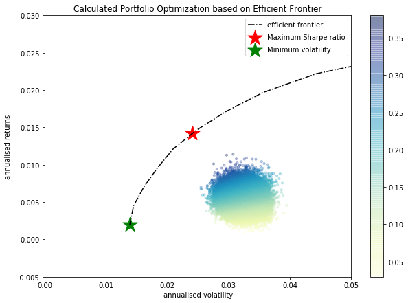
I understand the concept of the efficient frontier and am able to calculate it in Python. But even when generating 50'000 random 10 asset portfolios, the single portfolios are not even close to the efficient frontier.

I see that, for example, the maximum sharpe ratio portfolio has very pronounced allocation (most of the 10 asset get 0 allocation).

Since this work is very critical for myself I just wanted to ask the community if you experienced similar behaviour? Is it normal that when generating random portfolios not even one lies near the efficient frontier?

Please find the code below:

def portfolio_annualised_performance(weights, mean_returns, cov_matrix):
    returns = np.sum(mean_returns*weights )
    std = np.sqrt(np.dot(weights.T, np.dot(cov_matrix, weights)))
    return std, returns

def random_portfolios(num_portfolios, mean_returns, cov_matrix, risk_free_rate):
    results = np.zeros((3,num_portfolios))
    weights_record = []
    for i in range(num_portfolios):
        weights = abs(np.random.randn(len(mean_returns)))
        weights /= np.sum(weights)
        weights_record.append(weights)
        portfolio_std_dev, portfolio_return = portfolio_annualised_performance(weights, mean_returns, cov_matrix)
        results[0,i] = portfolio_std_dev
        results[1,i] = portfolio_return
        results[2,i] = (portfolio_return - risk_free_rate) / portfolio_std_dev
    return results, weights_record

def neg_sharpe_ratio(weights, mean_returns, cov_matrix, risk_free_rate):
    p_var, p_ret = portfolio_annualised_performance(weights, mean_returns, cov_matrix)
    return -(p_ret - risk_free_rate) / p_var

def max_sharpe_ratio(mean_returns, cov_matrix, risk_free_rate):
    num_assets = len(mean_returns)
    args = (mean_returns, cov_matrix, risk_free_rate)
    constraints = ({'type': 'eq', 'fun': lambda x: np.sum(x) - 1})
    bound = (0.0,1.0)
    bounds = tuple(bound for asset in range(num_assets))
    result = sco.minimize(neg_sharpe_ratio, num_assets*[1./num_assets,], args=args,
                        method='SLSQP', bounds=bounds, constraints=constraints)
    return result

def portfolio_volatility(weights, mean_returns, cov_matrix):
    return portfolio_annualised_performance(weights, mean_returns, cov_matrix)[0]

def min_variance(mean_returns, cov_matrix):
    num_assets = len(mean_returns)
    args = (mean_returns, cov_matrix)
    constraints = ({'type': 'eq', 'fun': lambda x: np.sum(x) - 1})
    bound = (0.0,1.0)
    bounds = tuple(bound for asset in range(num_assets))

    result = sco.minimize(portfolio_volatility, num_assets*[1./num_assets,], args=args,
                        method='SLSQP', bounds=bounds, constraints=constraints)
    return result

def efficient_return(mean_returns, cov_matrix, target):
    num_assets = len(mean_returns)
    args = (mean_returns, cov_matrix)

    def portfolio_return(weights):
        return portfolio_annualised_performance(weights, mean_returns, cov_matrix)[1]

    constraints = ({'type': 'eq', 'fun': lambda x: portfolio_return(x) - target},
                   {'type': 'eq', 'fun': lambda x: np.sum(x) - 1})
    bounds = tuple((0.0,1) for asset in range(num_assets))
    result = sco.minimize(portfolio_volatility, num_assets*[1./num_assets,], args=args, method='SLSQP', bounds=bounds, constraints=constraints)
    return result

def efficient_frontier(mean_returns, cov_matrix, returns_range):
    efficients = []
    for ret in returns_range:
        efficients.append(efficient_return(mean_returns, cov_matrix, ret))
    return efficients

def display_calculated_ef_with_random(mean_returns, cov_matrix, num_portfolios, risk_free_rate):
    results, _ = random_portfolios(num_portfolios,mean_returns, cov_matrix, risk_free_rate)
    
    max_sharpe = max_sharpe_ratio(mean_returns, cov_matrix, risk_free_rate)
    sdp, rp = portfolio_annualised_performance(max_sharpe['x'], mean_returns, cov_matrix)
    max_sharpe_allocation = pd.DataFrame(max_sharpe.x,index=curr_w_terms,columns=['allocation'])
    max_sharpe_allocation.allocation = [round(i*100,4)for i in max_sharpe_allocation.allocation]
    max_sharpe_allocation = max_sharpe_allocation.T

    min_vol = min_variance(mean_returns, cov_matrix)
    sdp_min, rp_min = portfolio_annualised_performance(min_vol['x'], mean_returns, cov_matrix)
    min_vol_allocation = pd.DataFrame(min_vol.x,index=curr_w_terms,columns=['allocation'])
    min_vol_allocation.allocation = [round(i*100,4)for i in min_vol_allocation.allocation]
    min_vol_allocation = min_vol_allocation.T
    
    print("-"*80)
    print("Maximum Sharpe Ratio Portfolio Allocation\n")
    print("Annualised Return:", round(rp,4))
    print("Annualised Volatility:", round(sdp,4))
    print("\n")
    print(max_sharpe_allocation)
    print("-"*80)
    print("Minimum Volatility Portfolio Allocation\n")
    print("Annualised Return:", round(rp_min,4))
    print("Annualised Volatility:", round(sdp_min,4))
    print("\n")
    print(min_vol_allocation)
    
    plt.figure(figsize=(10, 7))
    plt.scatter(results[0,:],results[1,:],c=results[2,:],cmap='YlGnBu', marker='o', s=10, alpha=0.3)
    plt.colorbar()
    plt.scatter(sdp,rp,marker='*',color='r',s=500, label='Maximum Sharpe ratio')
    plt.scatter(sdp_min,rp_min,marker='*',color='g',s=500, label='Minimum volatility')

    target = np.linspace(rp_min, 0.05, 20)
    efficient_portfolios = efficient_frontier(mean_returns, cov_matrix, target)
    plt.plot([p['fun'] for p in efficient_portfolios], target, linestyle='-.', color='black', label='efficient frontier')
    plt.title('Calculated Portfolio Optimization based on Efficient Frontier')
    plt.xlabel('annualised volatility')
    plt.ylabel('annualised returns')
    plt.legend(labelspacing=0.8)
    plt.ylim([-0.005,0.03])
    plt.xlim([0.0,0.05])

display_calculated_ef_with_random(log_ret, new_cov, 50000, 0)

I haven't annualised the Covar-Matrix since I already have annual return estimates as well as covar estimates.

My very question is: is this plausible or not?

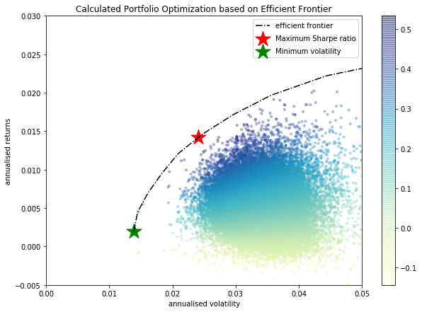
EDIT Since the weight generation process of my random portfolios seems to preffer too similar portfolio I changed the following function:

def random_portfolios(num_portfolios, mean_returns, cov_matrix, risk_free_rate):
    results = np.zeros((3,num_portfolios))
    weights_record = []
    for i in range(num_portfolios):
        weights = abs(np.random.randn(len(mean_returns)))
        weights[weights<1] = 0
        if sum(weights)==0:
            print("sum=0")
            indexes = np.unique(np.random.randint(0,10,3)).tolist()
            weights[indexes] = abs(np.random.randn(len(indexes)))
        weights /= np.sum(weights)
        weights_record.append(weights)
        portfolio_std_dev, portfolio_return = portfolio_annualised_performance(weights, mean_returns, cov_matrix)
        results[0,i] = portfolio_std_dev
        results[1,i] = portfolio_return
        results[2,i] = (portfolio_return - risk_free_rate) / portfolio_std_dev
    return results, weights_record

After doing so, the Portfolios are way better distributed:

So, can we then agree that the above code does what it should and I can continue from here?