Going through the literature on factor models, I keep seeing the phrase "dimensionality reduction" and how factor models allow for the modelling of assets in high-dimensional cases, and I would highly appreciate some explanation on how this works.
High dimensionality seems to occur when we attempt to model an entire asset universe (>1000, or $K$, assets, let's say) for optimal investment allocation, but there does not exist enough time-series data of $N$ data points for each asset, and standard techniques stop working when $N < K$. This is a clear issue.
Now, factor models try to explain an individual asset's return over time, $R_t$, with $k$ common factors $X_{k,t}$, through the basic model $$R_t = \beta_0 + \beta_1X_{1,t} + \beta_2X_{2,t} + \ldots + \beta_kX_{k,t} + \epsilon_t$$
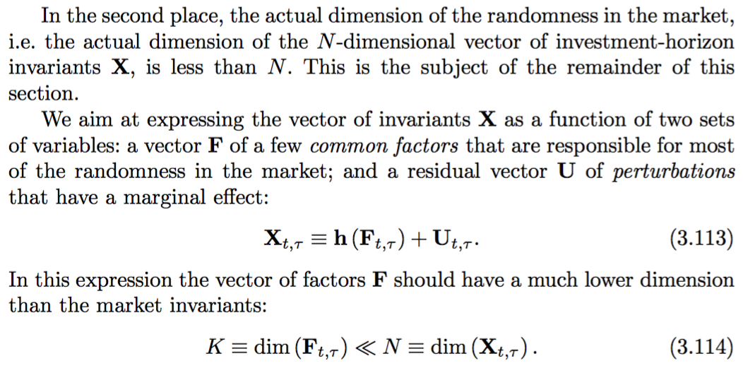
Succinctly put, how does such a model elaboration of $R_t$'s behavior reduce the dimensionality of the problem? There are still $K$ assets to model. Meucci's Risk and Asset Allocation (2005) describes it like this on pg. 132, without a satisfactory explanation (with $X$ being the returns and $F$ being the factors) ,
I hope someone can give the insight that explains this.
EDIT:
Could someone take me step by step through this imaginary example?
We have
- $K=20$ stocks,
- $N=10$ weekly price points for each (so a $N\times K$ matrix)
- $X=5$ factors shared among the 20 stocks (also 10 data points each)
Since the covariance of all the stocks cannot be calculated normally (since $N<K$), mathematically how does factor modelling recreate the covariance matrix?

