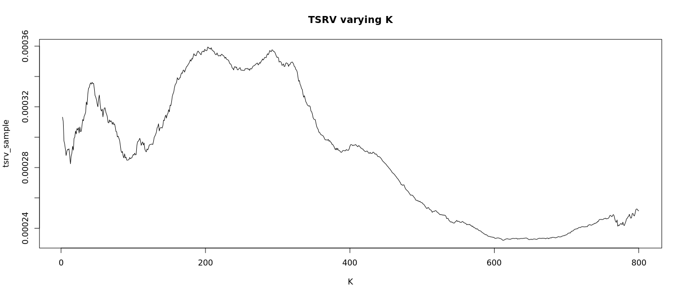
How to find optimal $K$?
If we let $i$ for $i=1,\ldots,n$ be the amount of intraday returns over a fixed interval $T$ (one day in empirical applications), then in Zhang et al. (2005) (p. 1397) specified above, they tell you that the optimal $c$, can be obtained via the equation:
\begin{equation}
c^{*} = \left(\frac{T}{12 \cdot \left(\mathbb{E}\left[\varepsilon_T^2\right]\right)^2} \cdot \int_{0}^{T} \sigma_s^4 \: ds\right)^{-\frac{1}{3}},
\end{equation}
where $\mathbb{E}\left[\varepsilon_T^2\right]$ is the variance of the noise process and can be found a couple of pages afterwards (p. 1404):
\begin{equation}
\widehat{\mathbb{E}\left[\varepsilon_T^2\right]} = \frac{1}{2n}\sum_{i=1}^n r_{i,T}^2,
\end{equation}
which was originally derived in the paper of Hansen and Lunde (2006). Furthermore, the integrated quarticity, $\int_{0}^T \sigma_s^4 \: ds$, can be estimated using the realized counterpart (be wary: noise and jumps under second-frequencies will affect the realized quarticity estimator):
\begin{equation}
RQ_T = \frac{n}{3}\sum_{i=1}^n r_{i,T}^4.
\end{equation}
How to find optimal J?
Reiterating from one of your own questions, the original paper does not work with any J subscript. However, their updated paper, Zhang et al. (2011) (p. 165) extend the TSRV estimator for dependent noise, where they further define the average lag j realized volatility and argue that it reduces to their original TSRV estimator for $J=1$:
We will continue to call this estimator the TSRV estimator, noting that the estimator we proposed in Zhang et al.(2005) is the special case where $J=1$ and $K\rightarrow \infty$ as $n\rightarrow\infty$.
To conclude, $J=1$ if you follow along Zhang et al. (2011) and $K=c n^{\frac{2}{3}}$ for $c$ being estimated as described above.

