Quantlib: day-by-day evaluation of option value

Question

I'm using Quantlib in Python to price an FX option. I'm comparing the result to Bloomberg, to make sure the code is working correct.

I want to calculate the P&L of a certain option trading strategy by using Taylor expansion of P&L (discussed in other post here) And also by using the NPV of the option.

Therefore, it's important to have a correct NPV for every date that the option is alive. The option I use to test this is a 1-week stylized option.

The problem that occurs is that the NPV matches Bloomberg correctly on the first, second, third and last date, but not on the other dates.

import QuantLib as ql


Spot = 1.1
Strike = 1.101
Sigma = 10/100
Ccy1Rate = 5/100
Ccy2Rate = 10/100
OptionType = ql.Option.Call

#Option dates in quantlib objects
EvaluationDate = ql.Date(3, 1,2022)
SettlementDate = ql.Date(5, 1, 2022) #Evaluation +2
ExpiryDate = ql.Date(10, 1, 2022) #Evaluation + term which is 1 week
DeliveryDate = ql.Date(12, 1, 2022) #Expiry +2
NumberOfDaysBetween = ExpiryDate - EvaluationDate
#print(NumberOfDaysBetween)

#Generate continuous interest rates
EurRate = Ccy1Rate
UsdRate = Ccy2Rate

#Create QuoteHandle objects. Easily to adapt later on.
#You can only access SimpleQuote objects. When you use setvalue, you can change it.
#These global variables will then be used in pricing the option.
#Everything will be adaptable except for the strike.
SpotGlobal = ql.SimpleQuote(Spot)
SpotHandle = ql.QuoteHandle(SpotGlobal)
VolGlobal = ql.SimpleQuote(Sigma)
VolHandle = ql.QuoteHandle(VolGlobal)
UsdRateGlobal = ql.SimpleQuote(UsdRate)
UsdRateHandle = ql.QuoteHandle(UsdRateGlobal)
EurRateGlobal = ql.SimpleQuote(EurRate)
EurRateHandle = ql.QuoteHandle(EurRateGlobal)

#Settings such as calendar, evaluationdate; daycount
Calendar = ql.UnitedStates()
ql.Settings.instance().evaluationDate = EvaluationDate
DayCountRate = ql.Actual360()
DayCountVolatility = ql.ActualActual()

#Create rate curves, vol surface and GK process
RiskFreeRateEUR = ql.YieldTermStructureHandle(ql.FlatForward(0, Calendar, EurRateHandle, DayCountRate))
RiskFreeRateUSD = ql.YieldTermStructureHandle(ql.FlatForward(0, Calendar, UsdRate, DayCountRate))
Volatility = ql.BlackVolTermStructureHandle(ql.BlackConstantVol(0, Calendar, VolHandle, DayCountVolatility))
GKProcess = ql.GarmanKohlagenProcess(SpotHandle, RiskFreeRateEUR, RiskFreeRateUSD, Volatility)

#Generate option
Payoff = ql.PlainVanillaPayoff(OptionType, Strike)
Exercise = ql.EuropeanExercise(ExpiryDate)
Option = ql.VanillaOption(Payoff, Exercise)
Option.setPricingEngine(ql.AnalyticEuropeanEngine(GKProcess))
BsPrice = Option.NPV()

ql.Settings.instance().includeReferenceDateEvents = True

ql.Settings.instance().evaluationDate = EvaluationDate
print("Premium is:", Option.NPV()*1000000/Spot)

ql.Settings.instance().evaluationDate = EvaluationDate+1
print("Premium is:", Option.NPV()*1000000/Spot)

ql.Settings.instance().evaluationDate = EvaluationDate+2
print("Premium is:", Option.NPV()*1000000/Spot)

ql.Settings.instance().evaluationDate = EvaluationDate+3
print("Premium is:", Option.NPV()*1000000/Spot)

ql.Settings.instance().evaluationDate = EvaluationDate+4
print("Premium is:", Option.NPV()*1000000/Spot)

ql.Settings.instance().evaluationDate = EvaluationDate+7
print("Premium is:", Option.NPV()*1000000/Spot)

Which results in:

Premium is: 5487.479999102207

Premium is: 5148.552323458257

Premium is: 4774.333578225227

Premium is: 4353.586300232529

Premium is: 3867.4561591587326

Premium is: 909.0909090908089

However, according to Bloomberg the premium should be:

5487.48 (correct)
5148.55 (correct)
4774.33 (correct)
4499.5 
4015.7
909.9 (correct)

The result on expiration is given by setting the following (the option expires in-the-money):

ql.Settings.instance().includeReferenceDateEvents = True

Can someone explain why the NPV suddenly doesn't match for those 2 dates?

Screenshots of option pricing in Bloomberg

Answer 1

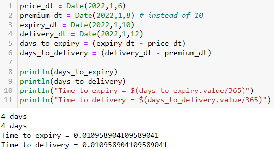
There are two different time gaps in OVML:

• time to expiry = Expiry Date - Price Date
• time to delivery = Delivery Date - Premium Date

You can see the premium date at the bottom of the OVML screen. Quantlib on the other hand does not distinguish price date and premium date (Matlab for example also doesn't distinguish this).

To illustrate this, I will use Julia because I already had this code. However, the syntax is sufficiently similar to Python so it should be possible to follow the logic. I replicate both Bloomberg's valuation and Quantlib's valuation to illustrate the differences.

Import all packages and define the cdf.

using Distributions, Dates
N(x) = cdf(Normal(0,1),x)

Define Dates

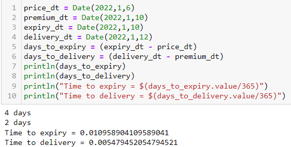
price_dt = Date(2022,1,6)
premium_dt = Date(2022,1,10)
expiry_dt = Date(2022,1,10)
delivery_dt = Date(2022,1,12)
days_to_expiry = (expiry_dt - price_dt)
days_to_delivery = (delivery_dt - premium_dt)
println(days_to_expiry)
println(days_to_delivery)
println("Time to expiry = $(days_to_expiry.value/365)")
println("Time to delivery = $(days_to_delivery.value/365)")

Result:

Define inputs

spot = 1.1
points = 3.06
fwd_scale = 10000
f = spot + points / fwd_scale
k = 1.101
ccy1 = 0.05 # EUR
ccy2 = 0.1 # USD
vol = 0.1
println(f)

Compute continuous interest rates (adjusted for differences in daycount between rates and vols)

r1_cont = log(1+ccy1*days_to_expiry/360)/(days_to_expiry/365)
r2_cont = log(1+ccy2*days_to_expiry/360)/(days_to_expiry/365)

Define Garman Kohlhagen with forward (technically Black76) => same result as can be seen here. Delivery is needed for discounting the put / call values.

function GKF(F,K, days_to_expiry, days_to_delivery ,ccy2,σ)
    d1 = ( log(F/K) +  0.5*σ^2*days_to_expiry.value/365 ) / (σ*sqrt(days_to_expiry.value/365))
    d2 = d1 - σ*sqrt(days_to_expiry.value/365)
    c  = exp(-ccy2*days_to_delivery.value/365)*(F*N(d1) - K*N(d2))
    p  =  exp(-ccy2*days_to_delivery.value/365)*(-F*N(-d1) + K*N(-d2))
  return c, p
end

Compute Option value (Julia has 1 based indexing). The division by spot is needed because standard GK is in terms of CCY2 (USD here). Notional is in CCY1, which means we need not change anything here.

Option = GKF(f, k, days_to_expiry, days_to_delivery, r2_cont, vol )
put = Option[2]*1000000/spot

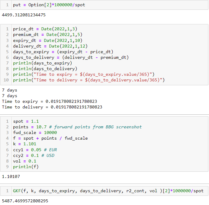
Result for the first day that is different, as well as the initial day to compare this.

There are minor rounding differences to BBG because I only used the fwd points visible in the screenshot, which lacks the exact decimal precision.

In case someone tries to replicate, the Quantlib code in the question should be (instead of .Call)

OptionType = ql.Option.Put

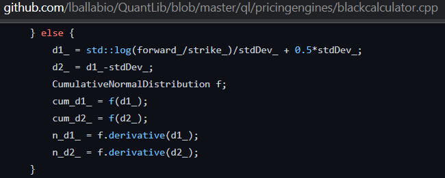
You can see the implementation of the code (in c++) here.

The same cpp file defines N()

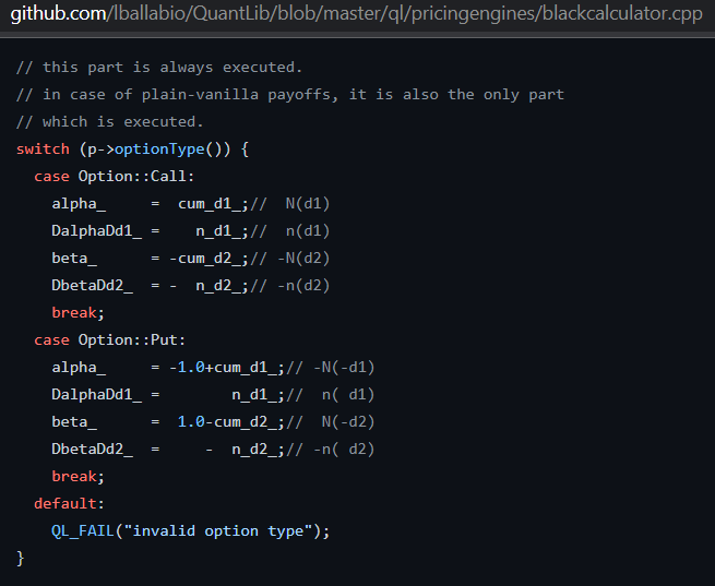
as well as how the actual value of the option is calculated

.

The crux here is that quantlib does not distinguish price date and premium date (in Bloomberg terminology). The forward is derived from the exchange rate on evaluation date, as well as the interest rate differential, adjusted for daycount. This can be done like so in Julia:

fwd = spot * exp((r2_cont - r1_cont)*days_to_delivery.value/365)

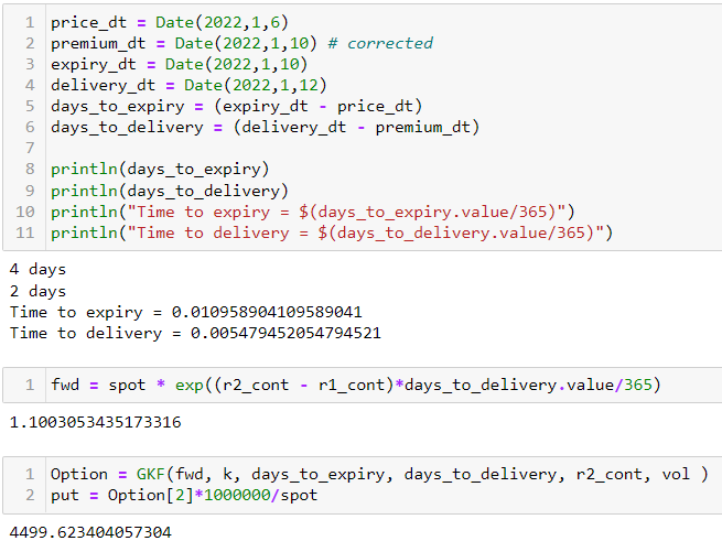
Now, following our above implementation, and knowing quantlib does not do this, we can simply set the premium date to always be T+2 (for EUR) and ignore any holidays / weekends (we could also just ignore the difference between price/premium as well as expiry/delivery).

With these dates, our forward is

and the option value as computed in quantlib is:

To cross check, if you were to now use the correct dates, you would get the BBG valuation.

Therefore, in quantlib, you cannot take into account settlement adjustment (e.g. T+2 for EURUSD, or T+1 for USDRUB), or compute delayed delivery (where delivery date is T+2, i.e. 2 days after expiry), as for example described in "Wystup, Uwe. FX options and structured products. John Wiley & Sons, 2015. p.26-29" or "Clark, Iain J. Foreign exchange option pricing: A practitioner's guide. John Wiley & Sons, 2011. p.33".

This is something Bloomberg or Murex offer.