Exercise 3.11 (Approximation of an Itô Integral). In this example, the stochastic integral $\int^t_0tW(t)dW(t)$ is considered. The expected value of the integral and the expected value of the square of the integral are estimated using $M=1,000,000$ sample paths. The number of intervals used on $[0,1]$ is $N$ where $N=4,8,16,\dots,256$. The preceding approximate method is used, which for this problem, has the explicit form \begin{align*} E((I(f))^\alpha)&=E\left(\int^1_0tW(t)dW(t)\right)^\alpha\\ &\approx\frac{1}{M}\sum^M_{j=1}\left(\sum^{N-1}_{i=0}t_i^{(N)}W^{(j)}(t_i^{(N)})(W^{(j)}(t^{(N)}_{t+1})-W^{(j)}(t^{(N)}_i))\right)^\alpha\quad(2)\\ \end{align*} for $\alpha=1$ or $2$ and $t_i^{(N)}=i/N$ for $i=0,1,2,\dots,N$. Notice that $(W^{(j)}(t^{(N)}_{i+1})-W^{(j)}(t_i^{(N)}))=\eta_i^{(j)}/\sqrt{N}$ where $\eta_i^{(j)}\sim N(0,1)$ and also that $(W^{(j)}(t^{(N)}_{i})-W^{(j)}(t_{i-1}^{(N)}))=\eta_{i-1}^{(j)}/\sqrt{N}$. A computer program that performs this calculation is listed at the end of this chapter. The calculational results are given in Table 3.2 for $M=1,000,000$ sample paths. Notice that the results improve as $N$ increases. The exact values are $E(I(f))=0$ and $E((I(f))^2)=0.25.$ \begin{array}{ccc} \hline \text{Value of N}&|E(I(f))|&|E((I(f))^2)|\\ \hline \color{red}{2^2}&\color{red}{0.00107}&\color{red}{0.14071}\\ 2^3&0.00012&0.19151\\ 2^4&0.00069&0.21906\\ 2^5&0.00038&0.23508\\ 2^6&0.00007&0.24209\\ 2^7&0.00001&0.24486\\ 2^8&0.00002&0.24821\\ \hline \end{array} Source: Modeling with Itô Stochastic Differential Equations by Edward Allen, pg. 74
My Question
Per Abezhiko's wonderful reply in my other question, one has $\mathbb{E}[X_t] = 0$, since $W_s$ and $\mathrm{d}W_s$ are independent and have zero mean, while Itô's isometry gives $$\mathrm{Var}[X_t] = \mathbb{E}[X_t^2] = \mathbb{E}\left[\int_0^t s^2W_s^2 \,\mathrm{d}s\right] = \int_0^t s^2\,\mathbb{E}[W_s^2] \,\mathrm{d}s = \int_0^t s^3 \,\mathrm{d}s = \frac{1}{4}t^4$$ which is equal to $1/4$ when $t=1$.
I've provided the Fortran code here from the textbook which was provided by the author, but I'd like to run this stochastic integral in python. There is a code which I used from here, to get the bottom values in the table, but the output is nonsense:
In [5]:
T = 1.0 # end time
N = 1000000 # number of steps, here it's
dt = T / N

dW = np.sqrt(dt) * np.random.randn(N)
W = np.cumsum(dW)

shiftedW = np.zeros(N)
shiftedW[1:] = W[:-1]

# The two different integrals.
# The Ito integral is roughly the Riemann integral evaluated at the left edge of the subinterval
ito = np.sum(shiftedW*dW)
# The Stratonovich integral is roughly the Riemann integral evaluated at the centre of the subinterval
stratonovich = np.sum((0.5*(shiftedW+W) + 0.5*np.sqrt(dt)*np.random.randn(N))*dW)

# Note that the exact solutions are different - markedly so!
print("The Ito integral is {} with error {}".format(ito, np.abs(ito - 0.5*(W[-1]**2-T))))
print("The Stratonovich integral is {} with error {}".format(stratonovich, np.abs(stratonovich - 0.5*W[-1]**2)))

## The Ito integral is 2.264544487686194 with error 0.0008807299528790224
## The Stratonovich integral is 2.765668595686916 with error 0.00024337804784302364

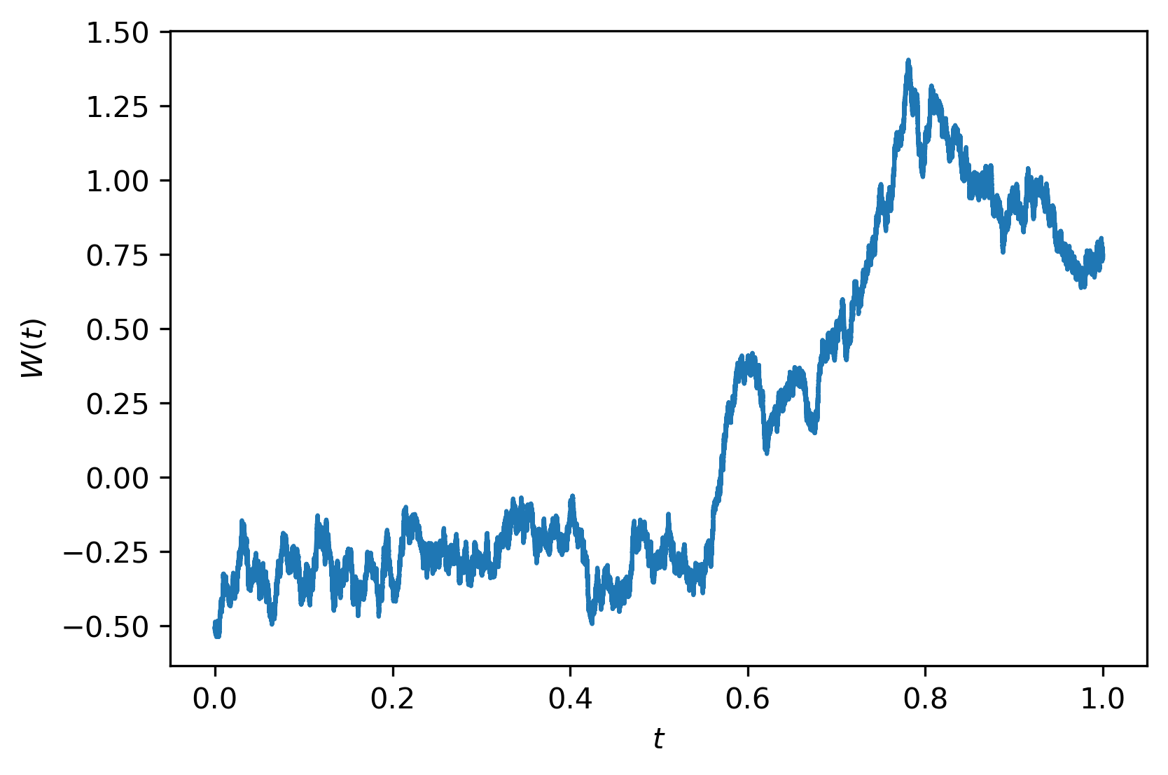
plt.plot(t, W)
plt.xlabel(r'$t$')
plt.ylabel(r'$W(t)$')
plt.savefig('itointegral', dpi=300, bbox_inches='tight')
plt.show()
Would anybody be able to provide a hint?

