When optimizing a portfolio for risk parity, can any portfolio weights turn negative?

Question

As the title reads, when performing risk parity optimization (equal risk contribution amongst all assets to the portfolio volatility), is it possible for weights to turn negative?

I understand that in the regular portfolio optimization, it is necessary to set a short sales restriction, if not it is possible to have negative weights in the mean-variance optimization or the "burst" of weights.

However, I saw that in packages of R such as "riskParityPortfolio" there isn't a selection for short sale restrictions. Does that mean that the risk parity optimization inherently does not result in negative weights?

Answer 1

Many risk-parity implementations simply use the inverse-vol rule (i.e. weights are proportional to 1 over vol), and then all weights are (strictly) positive by construction.

A number of implementations that do the full optimization indeed set non-negativity as an explicit constraint. But in general and without such constraints, negative weights may occur when you equalize risk-contributions (though negative weights may be unlikely).

An example in R for a 4-by-4 covariance matrix, which is of rank 4 and positive definite:

S <- structure(c(0.000366309632978563, -0.000105943107569848,
                 -0.000119667135542588, 0.000169622848883779,
                 -0.000105943107569848, 0.000187730511335559,
                 -6.49497066288097e-05, -0.000167162505503921,
                 -0.000119667135542588, -6.49497066288097e-05,
                 0.000102201079006482, 1.88829418811814e-05,
                 0.000169622848883779, -0.000167162505503921,
                 1.88829418811814e-05, 0.000208993337170307),
               dim = c(4L, 4L))

The implied correlation matrix:

cov2cor(S)
##        [,1]   [,2]   [,3]   [,4]
## [1,]  1.000 -0.404 -0.618  0.613
## [2,] -0.404  1.000 -0.469 -0.844
## [3,] -0.618 -0.469  1.000  0.129
## [4,]  0.613 -0.844  0.129  1.000

I do not use the riskParityPortfolio package, but it seems to support negative weights, though the default is to not allow them:

library("riskParityPortfolio")
riskParityPortfolio(S)
## $w
## [1] 0.2313 0.2990 0.4588 0.0109
## 
## $relative_risk_contribution
## [1] -1.9471 -0.0858  1.5197  1.5132
## ....


riskParityPortfolio(S, w_lb = -1)
## $risk_concentration
## [1] 1.93e-14
## 
## $w
## [1] -0.0829  0.4391  0.2167  0.4271
## 
## $relative_risk_contribution
## [1] 0.25 0.25 0.25 0.25
## ....

---

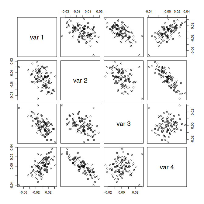
Additional note: The example covariance-matrix hides some fairly-strong dependencies between the asset returns, which may not be obvious from looking at the data:

library("NMOF")
R <- randomReturns(na = 4, ns = 100,
                   sd = sqrt(diag(S)),
                   rho = cov2cor(S), exact = TRUE)
pairs(R)

Computations based on such a matrix (such as a marginal-risk calculation) will typically be sensitive and react strongly to small changes ("perturbations") of inputs. In the example, you can get around this by increasing the iterations:

w <- riskParityPortfolio(S)$w
FRAPO::mrc(w, S)
## [1] -194.71   -8.58  151.97  151.32

w <- riskParityPortfolio(S, maxiter = 1e4)$w
FRAPO::mrc(w, S)
## [1] -67.3  11.2  78.2  77.9

w <- riskParityPortfolio(S, maxiter = 1e5)$w
FRAPO::mrc(w, S)
## [1] 23.1 24.7 26.1 26.1

w <- riskParityPortfolio(S, maxiter = 1e6)$w
FRAPO::mrc(w, S)
## [1] 25 25 25 25

(I use the marginal-risk function mrc from Bernhard Pfaff's FRAPO package.) But of course, this is all the result of an empirical problem (not a computational one): the assets are highly-correlated, and so an algorithm will always have trouble differentiating between linear combinations of those assets.