Why is asset volatility easier to estimate than the asset mean if it contains the mean?

Question

It is well known that the variance of asset returns, $\sigma^2$ (whose square root is volatility), is easier to estimate than the asset mean $\mu$ (also known as expected return) because the mean of asset returns is very difficult to estimate.

Why is this the case, given that the sample estimator for volatility itself contains the sample estimator of the asset mean in its formula?

$$\hat{\sigma} = \sqrt{\sum_{i=1}^n \frac{(x_i-\hat{\mu})^2}{n-1}}$$

Shouldn't the estimation error from $\hat{\mu}$ seep into the estimation error of $\hat{\sigma}$? If not, why doesn't it?

Answer 1

Let me add two points to Quantoisseur's answer.

Standard Errors

The difference between estimating variances and means is that the standard error of the variance estimator depends on the size of the sample (number of observations), whereas the standard error of the mean depends on the length (or duration) of the sample, see here. So, if you use finer and finer data points (up to high frequency data), you typically improve the accuracy of the variance estimator (see, for example, realised variance) but not the accuracy of the mean estimator. For the latter, you have to extend the estimation sample (time horizon) as a whole.

Autocorrelation

Let's talk about conditional mean and variance. Please look at the autocorrelation plots of IBM's returns below. As you see, the returns themselves hardly depict any significant autocorrelation. Thus, you cannot really use historical data to forecast future expected returns. However, squared returns (which proxy the unobservable variance) depict significant autocorrelation. Thus, historical squared returns carry some information about future conditional variances. That's why GARCH models work: squared returns are autocorrelated. Recall that $\mathrm{Var}[R]=\mathrm{E}[R^2]-\mathrm{E}[R]^2\approx \mathrm{E}[R^2]$.

Impact of Mean on Variance Estimation

My first point with the standard error is that we can't estimate the mean of a time series of returns accurately. It may be 1% or 3% or -2% (often we can't even be sure about the sign!). All are very well possible. But does it matter for the variance? By definition, $\mathrm{Var}[R]=\mathrm{E}[(R-\mathrm{E}[R])^2]=\mathrm{E}[R^2]-\mathrm{E}[R]^2$. Now, if you square 0.01, 0.03 or -0.02, you get negligible numbers. So, despite having potentially huge standard errors in the mean estimation (3% is kind of three times as big as 1%), it doesn't really impact the estimation of the variance because the variance deals with squared quantities and returns are sufficiently close to zero.

Answer 2

The answer is not statistical. In almost every other area of statistics, estimating the mean is easier (i.e. it can be estimated with higher precision) and estimating higher moments like variance (and thus volatility), skewness, kurtosis, etc. is harder -- sometimes much harder.

The key points that make financial statistics (or financial econometrics, if you prefer) different are market efficiency and competition.

Market Efficiency

An efficient market is one where all prices are fair: you cannot find prices which are clearly wrong in light of risk.

How do markets become efficient? Suppose you knew a stock was going up. You would buy the stock -- until doing so no longer was expected to make money. The same goes for shorting a stock you knew would fall. If your information were not guaranteed, you might still take some risk by buying or selling (though maybe less so). Therefore, your trading also is tempered by uncertainty.

Competition

You are not the only person trying to make money; other people are also always looking for information that will help them make money. If two or more people learn of some information, the first person to trade and move prices will earn money while the late person will earn no money. That makes people compete to be the first to trade on information. Over all of the people in the market, that means prices quickly incorporate new information.

Apart from the times when people get new information, prices are fair: they have incorporated all of the information. When new information arrives, people trade on that to make money which changes prices... until prices are again fair. Competition makes market prices fair and fair prices make the market efficient.

Predicting the Mean

The result is that predicting the movement of a stock is difficult, especially most of the time when you lack information. Furthermore, we think prices adjust rapidly to new information so most of the time we do not know where prices will go next.

Sure, you expect to get a return at least as good as the risk-free rate, but how much more? That is difficult to determine. If it were not difficult to determine, you would be back to trading until prices were fair.

Together, these economic realities have two implications. First, predicting the mean return of a stock is difficult. If it were not so, trading and making money would be easy. Second, guessing when a stock will move a lot is even more difficult; hence most investors say it is easier to just hold a stock for a long period of time and (hopefully) benefit from those changes instead of trying to time them.

Volatility

So now we can understand why predicting the mean return is difficult. It is not so much that predicting volatility is easy but more that predicting volatility is easier than predicting the mean for asset returns.

At this point, you might say "but then why can't I make easy money trading the VIX?" (or other volatility-related instruments). Competition and market efficiency again make that difficult: those forces keep the VIX and other volatility-related instruments fairly priced. That helps us make better estimates of volatility over long stretches of time: hours, days, months, and so on.

However, if you tried to predict the VIX over minutes and trade on that... you would likely find it just as difficult as predicting stock returns.

Answer 3

A simpler answer is thus. There are known historical values for the past year for the mean. It's simply the end of year value divided by the beginning value.

However, we can't improve the estimate of the mean by looking at, say, the daily returns and aggregating them up to 250 days of trading to make a better estimate of the mean (return): it will simply end up being those two values divided.

However, with variance (or stdev) we CAN look at weekly values and average them to get a better read on the value than we can by looking at monthly data, etc..

Answer 4

The sample variance and standard deviation (volatility) formulas are:

If your question is why is volatility easier to predict than returns, the intuitive answer is because the numerator is squared and thus has only positive values. This simplifies the problem as now I don't have to worry about predicting the sign of the return, only the size.

Answer 5

In fact, a standard way to estimate the volatility does not use the mean at all (the mean is set to zero in the formula), because, as pointed out in @Kevin's answer, it really makes no difference, so the premise of the question is a bit fraught. It should be noted that the market mean return is extremely robust (and very close to constant, at around 4 basis points per day) over very long periods (as in, several decades), so the answer to the question depends on what time horizon you are looking at.

Answer 6

This is largely because the variance of stock returns is high relative to their mean.

The idea that stock return means are harder to estimate is old and was already known before high frequency data, or even GARCH models, were widely used. The point is made e.g. in this 85 paper by Jorion who writes:

On the other hand, uncertainty in variances and covariances is not as critical because they are more precisely estimated

However, I believe the point is even older.

Let me consider a simple example. Assume stock returns are i.i.d. and follow a normal distribution $r \sim N(\mu, \sigma^2)$, where both the mean and variance are unknown. The standard confidence interval for the mean is

$$[\hat{\mu} - t_{n-1,\alpha/2}\frac{s}{\sqrt{n}},\hat{\mu} + t_{n-1,\alpha/2}\frac{s}{\sqrt{n}}],$$

where $t_{n-1,\alpha/2}$ is the $\alpha/2$-percentile t-stat with $n-1$ degrees of freedom. The confidence interval for standard deviation uses the chi-square distribution and is given by (see here)`

$$\left[\sqrt{\frac{(n-1)s^2}{\chi^2_{n-1,\alpha/2}}},\sqrt{\frac{(n-1)s^2}{\chi^2_{n-1,1-\alpha/2}}}\right].$$

Consider the monthly returns of the S&P 500 (long-run mean roughly $0.8\%$ and standard deviation $4.5\%$). Assume you sample 20 years of returns, i.e. $n=240$. Assume your estimators happen to get the mean and standard deviation correct. Now the $95\%$-confidence interval for mean becomes

$$[0.23,1.37].$$

The confidence interval for the standard deviation becomes

$$[4.13,4.94].$$

You can see that the confidence interval for standard deviation is relatively tighter. But this is not the case for arbitrary values of mean and standard deviation. Rather the stock return mean and standard deviation happen to be such that the latter bound is relatively tighter because the mean is low relative to standard deviation.

If you increase the stock return mean to say $10\%$ monthly holding standard deviation constant, the confidence interval for mean becomes relative tigher than that for the standard deviation. If you look at any other normal distribution, you might easily find that you estimate the mean with greater precision than standard deviation. As the answer by kurtosis suggests, in other contexts, means are often easier to estimate than variances.

Answer 7

I am reading this 2.5 months after the question was asked but I still see some confusion in the answers (or at least I am confused by them).

1. The OP claims that the variance of asset returns is easier to estimate than the mean, but the statement is not formulated mathematically. The currently available answers do not formulate it mathematically either. This makes a rigorous discussion difficult.
2. More specifically, the central concepts are mean and variance of asset returns. Theoretical mean (mathematical expectation) and variance only make sense as parameters of a statistical/probabilistic model of the data generating process (DGP). The model is not given by the OP nor by the currently available answers. Without a rigorous definition of the estimand, a discussion of ease of estimation is problematic.
3. Moreover, neither the OP nor the currently available answers define estimation precision mathematically nor provide formulas of estimation precision for mean and variance.
4. Even when the theoretical mean and variance are well defined mathematically, they are not observed. Thus, evaluating estimation precision is nontrivial; we cannot just compare the estimate to the actual value since the latter is latent. At least some answers seem to conflate the observed realization of an asset return with the theoretical mean of the underlying distribution. (However, there may be models that define variance in terms of observed data, and then variance might be observed given the relevant data.)
5. In a similar vein, estimation of mean is not the same as point prediction. Point prediction can be hard if variance is large even if the theoretical mean is known. Therefore, large prediction errors do imply the mean has been estimated poorly.

While this does not answer the OPs question directly, it hope it guides the discussion towards a rigorous answer.

Update: see a related question here.

Answer 8

I would like to posit a more straightforward answer, it is a mathematical illusion.

Although this can be solved through formal theory because the distributions are known, doing so would create a long post. Instead, it can be quickly illustrated through a simulation.

Let us assume that the data are normally distributed. The results depend on that. If they are drawn from a different distribution, then the standard deviation's correction factor will change. The assumption that I am using is that the observations are independent because your formula implies it. This correction would not work for autocorrelated data. Nonetheless, the illustration would work out the same in the end, and independence means less work for me.

The unbiased estimate of the mean is $$\bar{x}=\frac{\sum_1^Nx_i}{N}.$$

The unbiased estimate of the variance is $$s^2=\frac{\sum_1^N(x_i-\bar{x})^2}{N-1}$$

The unbiased estimate of the standard deviation is $$s=\frac{\sqrt{ \frac{\sum_1^N(x_i-\bar{x})^2}{N-1}}}{\sqrt{\frac{2}{N-1}}\frac{\Gamma(\frac{N}{2})}{\Gamma(\frac{N-1}{2})}}$$

The correction factor is needed because the sampling distribution of the unbiased estimate of the variance is Snedecor's F distribution. In contrast, the sampling distribution of the unbiased estimate of the standard deviation is the Chi distribution. The square root of the unbiased estimator of the sample variance is a biased estimator of the standard deviation.

What I did was create 100,000 samples, each with 1,000 observations, from a standard normal distribution. The code is at the bottom of the answer.

I then calculated the unbiased estimates of the mean, variance, and standard deviation. The distribution of each one is the sampling distribution of the mean, variance, and the standard deviation. So there is now a sample of each with 100,000 observed parameter estimates for each category.

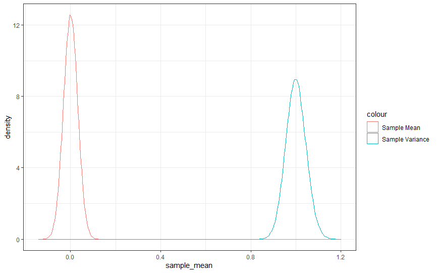
Suppose you look graphically at the sampling distribution of the mean and the variance. In that case, you will see that the distribution of the estimator for the population mean is denser than for the population variance. Of course, you could be more precise by creating descriptive statistics for each estimator.

The sampling distribution of the mean is Student's distribution, but the sample is so large that it will have converged to the normal for any practical purpose. The sampling distribution of the variance is Snedecor's F distribution, so though they look quite a bit alike, they really are different things.

Nonetheless, it would appear that the estimator of the mean is more precise than the estimator of the variance. That should be unsurprising because the estimator of the mean is buried inside the estimator of the variance. There are two sources of error.

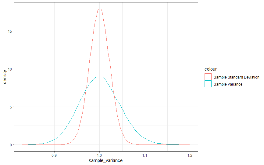
In this example, the mean's observed squared error is approximately 100 units and of the variance 200 units. So what happens when we compare the squared error of the variance and the standard deviation? The squared error of the standard deviation is approximately 50. Visually, you can see that in the graph below.

However, this is an illusion, and what should make you suspicious is the missing change of units intrinsic to this way of looking at the problem. You could make all kinds of transformations with the data or the statistics aside from the square root divided by a correction factor. Each one would stretch or shrink the estimation relative to the variance or the mean. It would not imply that they would improve the precision of the estimate.

Note that the above does not imply that there does not exist a transformation or different function that would improve precision or cause an estimator to behave better under some circumstances. Here, though, it is an illusion.

EDIT In response to a comment, I thought I would point out why this question is problematic. Consider a vector $$\theta=\begin{bmatrix}a \\ b\\ c\end{bmatrix}$$ and a second vector $$\theta'=\begin{bmatrix}d\\ e\\ f\end{bmatrix}$$ that may be estimators for some true parameter $\Theta$.

Let us also assume that $\theta\succ\theta'$ under some standard of optimality. Here that standard is that it minimizes the variance of the estimate and it is unbiased. That is far from the only standards that could be used.

It isn't meaningful to talk about the precision of estimation of $a$ versus $b$ in the vector $\theta$, even if one is a transform of the other under the algorithm. I would point out that $s^2$ is a transformation of $\bar{x}$. Each one is estimated in the best way possible under the criteria.

It may be meaningful to discuss the precision and accuracy differences between $a$ and $d$ but not between $a$ and $b$.

The only exception to that case is if a different objective function is chosen. To give an example, if an all-or-nothing loss function were used instead of quadratic loss, the estimator of both the variance and the standard deviation would be improved in precision, though with a loss of accuracy.

If the average loss were used instead of minimizing maximum risk, which is how most Frequentist estimators are chosen, you would get possibly quite different outcomes as well. Indeed, they could not be first-order stochastically dominated by the Frequentist estimators, though they could tie.

If you are finding one easier than another, there is some assumption being strongly violated somewhere. Something else is going on that is being missed and it could be very important.

I, of course, have strong opinions on what that is, but that is not the question presented.

rm(list = ls())
library(ggplot2)

set.seed(500)

observations<-1000
experiments<-100000

x<-matrix(rnorm(observations*experiments),nrow = observations)

sample_mean<-apply(x,2,mean)
sample_variance<-apply(x,2,var)

correction_factor<-exp(log(sqrt(2/(observations-1)))+lgamma(observations/2)- lgamma((observations-1)/2))

sample_standard_deviation<-sqrt(sample_variance)/correction_factor

Frequentist_estimators<-data.frame(sample_mean=sample_mean,sample_variance=sample_variance, 
 sample_standard_deviation=sample_standard_deviation)
rm(sample_mean)
rm(sample_variance)
rm(sample_standard_deviation)



Frequentist_errors<-data.frame(mean_error=(Frequentist_estimators$sample_mean)**2,variance_error=(Frequentist_estimators$sample_variance-1)**2,sd_error=(Frequentist_estimators$sample_standard_deviation-1)**2)

a<-ggplot(Frequentist_estimators)+theme_bw()
b<-a+geom_density(aes(sample_mean,colour="Sample Mean"))+geom_density(aes(sample_variance,colour="Sample Variance"))

print(b)

a<-ggplot(Frequentist_estimators)+theme_bw()
b<-a+geom_density(aes(sample_variance,colour="Sample Variance"))+geom_density(aes(sample_standard_deviation,colour="Sample Standard Deviation"))

print(b)

print(paste0("Observed Squared Error of the Mean is ",sum(Frequentist_errors$mean_error)))


print(paste0("Observed Squared Errors of the Variance is ",sum(Frequentist_errors$variance_error)))

print(paste0("Observed Squared Error of the Standard Deviation is ",sum(Frequentist_errors$sd_error)))

Answer 9

Similar to what eSurfsnake said: Actually, it is because you can estimate the variance exactly if you increase the sampling frequency enough (given that you use time-series data). This is the idea behind using intraday data to estimate realized variances, for example.

But the mean estimate cannot be improved by simply increasing the sampling frequency. As you increase the frequency from year, to month, to day, to hour, the standard errors increase in proportion. So you gain nothing. In this case, your only alternative is to get a longer sample.