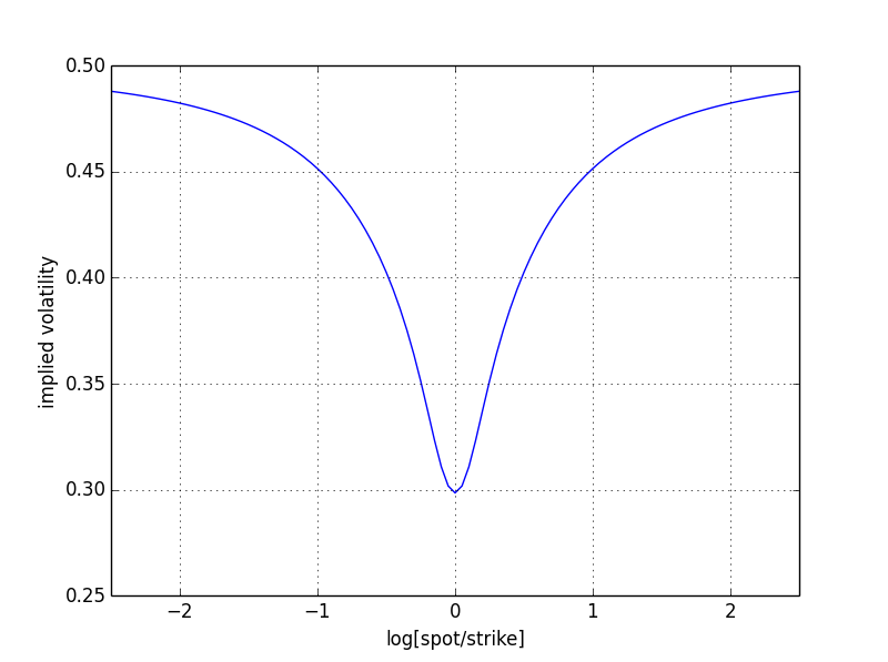
It is not the fact that volatility is time varying that creates the skew per se, but the fact that volatility is negatively correlated with the spot. That is to say, as the stock/index price declines volatility will tend on average to increase, and vice versa. Time varying volatility itself would create a more symmetric 'smile'.
Edit:
Suppose that you have a very simple case where volatility can take only two values $(\sigma_L,\sigma_H) = (0.10,0.50)$ with 50-50 probability. Also say that the drift is zero under both regimes. This is the simplest case of 'stochastic volatility,' if you want.
Then, the price of the option will just be the 50-50 weighted average of the two Black-Scholes prices
$$ C = 0.5\ BS(S,X,r,\sigma_L,T)+0.5\ BS(S,X,r,\sigma_H,T) $$
Equivalently, the risk neutral distribution of the log-price will be the 50-50 mixture of two Gaussians with different volatilities which exhibits fat tails.
Intuitively, when you are at the money both parts of the weighted sum contribute to the uncertainty, and the implied vol is roughly the average of the two vols, around 0.30. A Gaussian with this volatility will exhibit practically zero probability mass beyond $\pm 1.8$ which is the 6-sigma event point. However, the 50-50 mixture still has some considerable mass, since for the high volatility regime this is only a 3.5-sigma event. To mimic this mass a higher implied vol is required. This is symmetric, hence a 'smile'.
You can see that graphically below, where I have calculated the implied volatility for this example.

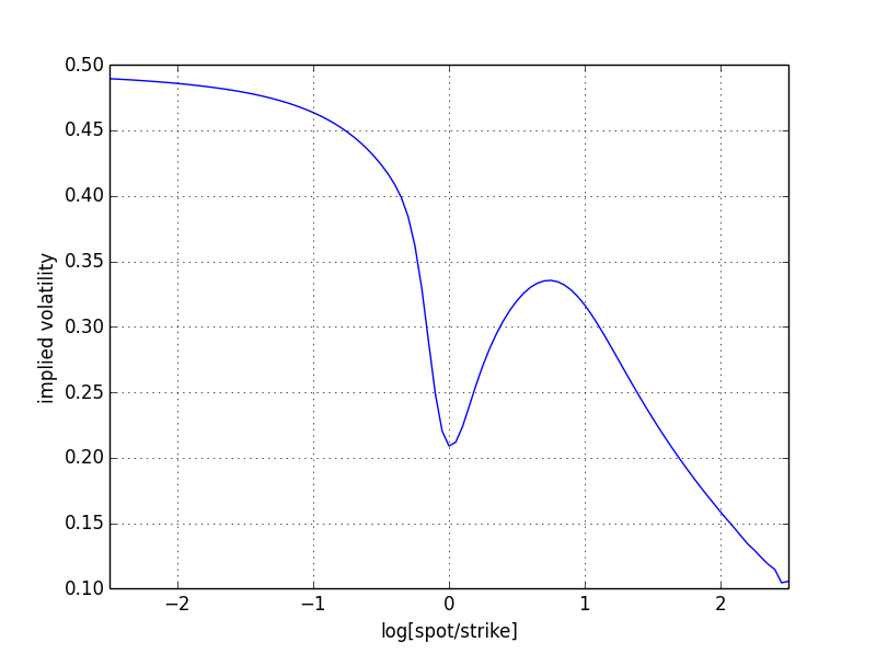
Now suppose that we have a 'negative correlation', that is to say we still have a 50-50 mixture but now when vol takes the 'low' value 0.10 then the drift is +0.10 positive, but when vol takes the 'high' value of 0.50 then the drift is -0.10 negative.
In that case the +6-sigma event is not symmetric to the -6-sigma event. In fact, implied vol on one side will converge to the 'high' vol of 0.50 while the other side will converge to the 'low' vol of 0.10, following the drifts. Hence we are presented with a 'skew' rather than a 'smile'
 .
.
Ok, this picture looks a bit odd! This is due to the extreme parameter values in the example, and reflects the 'weight' each distribution has in the mixture at each point. In any case, here is the Python code that created the pics to play with.
# parameters
sH = 0.50 # High vol regime
mH =-0.10 # Drift in high vol regime
sL = 0.10 # Low vol regime
mL =+0.10 # Drift in low vol regime
wH = 0.50 # Mixing weight

# code
import numpy as np
from scipy.stats import norm
from scipy.optimize import root
import matplotlib.pyplot as plt

N = norm(0,1).cdf
n = norm(0,1).pdf

def bs(S, X, r, sigma, T):
    d1 = np.log(S/X)+(r+0.5*sigma*sigma)*T
    d1 = d1/sigma/np.sqrt(T+1E-10)
    d2 = d1 -sigma*np.sqrt(T)
    return S*N(d1) -X*np.exp(r*T)*N(d2)
def iv(S, X, r, T, C):
    return root(lambda s: bs(S, X, r, s, T)-C, 0.50*np.ones(C.shape)).x

L = 2.5
X = 100.*np.exp(np.linspace(-L, L, 101))
cH = bs(100., X, mH, sH, 1.)
cL = bs(100., X, mL, sL, 1.)
c = wH*cH+(1-wH)*cL

m =np.log1p(wH*(np.exp(mH)-1)+(1-wH)*(np.exp(mL)-1))
v = iv(100., X, m, 1., c)

fg = plt.figure()
ax = fg.add_subplot(111)
ax.plot(np.log(100./X), v)
ax.set_xlim(-L, L)
ax.set_xlabel('log[spot/strike]')
ax.set_ylabel('implied volatility')
ax.grid()


