3
$\begingroup$

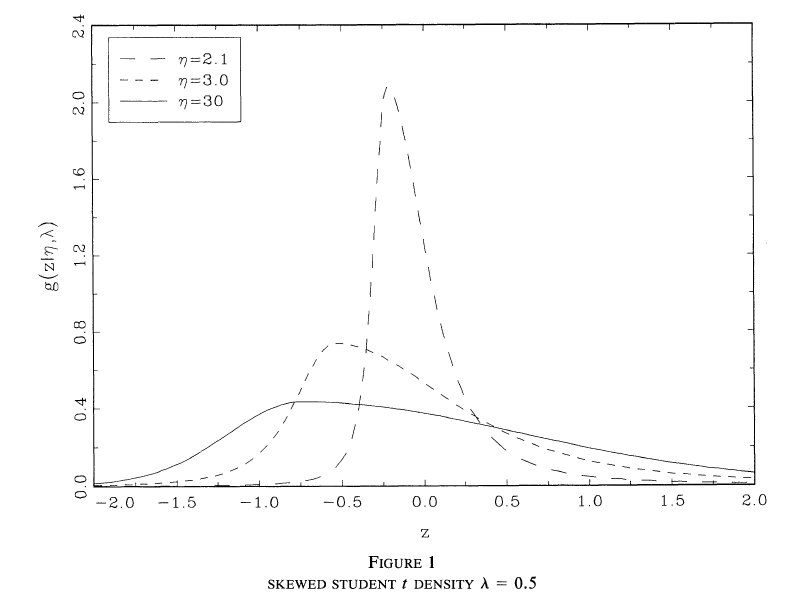
I am using the sgt package in R to recreate the plot from Hansen's paper ( available here http://www.ssc.wisc.edu/~bhansen/papers/ier_94.pdf on page 8) using random draws from the skew-t distribution.

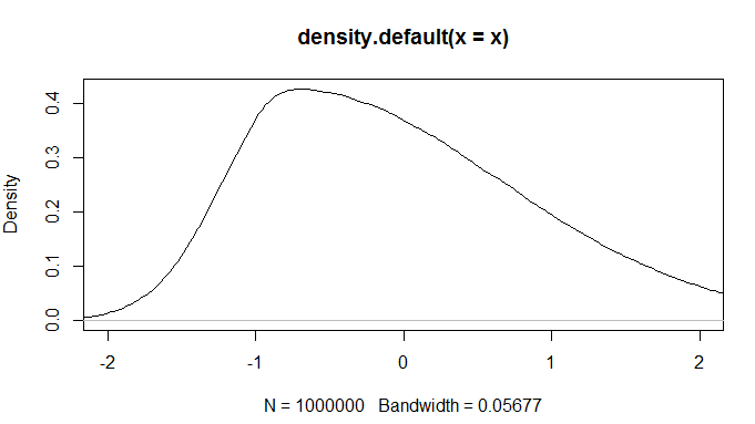
I begin with $\eta=30$ using the following code:

x = rsgt(1000000, mu = 0, sigma = 1, lambda = 0.5, p = 2, q=30, mean.cent=TRUE, var.adj=TRUE)
t=density(x)
plot(t, xlim=c(-2, 2))

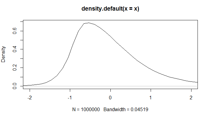
And I obtain a plot that is analogycal to the one given in the paper. However, using $\eta = 3$ or $\eta = 2.1$ (replace q with one of those values) results in much different plots, which look weird. Do you have any suggestions to how to solve this matter?

Edit: I include the plots I want to obtain and the ones I can obtain.

Plot from Hansen's paper

The one for $\eta=30$: enter image description here

The one for $\eta=2.1$: enter image description here

$\endgroup$
1
  • $\begingroup$ It would be helpful if you could post the resulting plots here. $\endgroup$
    – vonjd
    Commented Feb 23, 2016 at 8:31

1 Answer 1

3
$\begingroup$

The rsgt is a skewed generalized t distribution, whereas your picture is a skewed student-t distribution. Try using fGarch package.

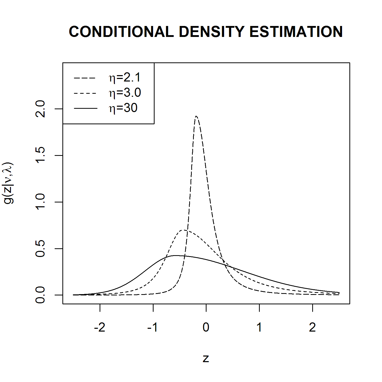
Plot reproduced:

library(fGarch)
x<-seq(-2.5, +2.5, by=0.001)
plot(x,
     fGarch::dsstd(x, mean = 0, sd = 1, nu = 30, xi = 1 + 0.5),
     type = "l",
     ylim=c(0, 2.4), lty = 1,
     xlab="z",
     ylab=expression(paste("g(z|",nu,",",lambda,")")),
     main="CONDITIONAL DENSITY ESTIMATION")

lines(x,
      fGarch::dsstd(x, mean = 0, sd = 1, nu = 3.0, xi = 1 + 0.5),
      type = "l",
      ylim=c(0, 2.4),
      lty = 2)

lines(x,
      fGarch::dsstd(x, mean = 0, sd = 1, nu = 2.1, xi = 1 + 0.5),
      type = "l",
      ylim=c(0, 2.4),
      lty = 5)

legend(x="topleft", legend = c(expression(paste(eta,"=2.1")),
                               expression(paste(eta,"=3.0")),
                               expression(paste(eta,"=30"))),
       lty=c(5,2,1))

enter image description here

$\endgroup$
4
  • $\begingroup$ Many thanks for this solution! One more question: Why are you using xi = 1 + 0.5 instead of $0.5$? Because I was under the impression that this version of the skew-t Distribution by Fernandez and Steel is different from the one of Hansen. $\endgroup$
    – Masher
    Commented Feb 23, 2016 at 21:02
  • $\begingroup$ And why could I obtain the plot for $\eta = 30$ using the method proposed by me and not the other values? Is my random sampling wrong? I am also interested in random sampling from this distribution, that is why this is important to me. $\endgroup$
    – Masher
    Commented Feb 23, 2016 at 21:16
  • 1
    $\begingroup$ the $alpha=0.5$ is a right skew, but for sstd the xi=1 is no skew, so making it right-skew, you need to add the +0.5 $\endgroup$
    – rbm
    Commented Feb 24, 2016 at 20:47
  • $\begingroup$ Thank you! And could you tell me what is wrong with my method for other values of the parameters, as for $\eta = 30$ the method I described seems to work just fine. $\endgroup$
    – Masher
    Commented Feb 24, 2016 at 21:00

Your Answer

By clicking “Post Your Answer”, you agree to our terms of service and acknowledge you have read our privacy policy.

Not the answer you're looking for? Browse other questions tagged or ask your own question.