Max option leverage strike

Question

Since options represent leveraged stock investments, at which strike $K$ does a European option provide maximum leverage?

Hereby define leverage $L$ as ratio of Delta/Optionprice:

$$L(K)=\frac{\Delta(K)}{C(K)}$$

You can assume all parameters fixed and positive ($T-t>0$) except strike $K (>0)$.

Delta is defined as $\Delta=\frac{\partial C(S)}{\partial S}$.

The maximum option leverage strike is important as it provides the maximum possible profit (and loss) on investment.

---

• Numerical solutions would be acceptable (e.g. MATLAB fmincon).

• Graphical solutions would also be acceptable (e.g. MATLAB plot or http://www.wolframalpha.com/input/?i=x%5E2).

• Intuitive explanations would be acceptable.

• For theoretical solutions you can use Black-Scholes model where

\begin{align} C(S, t) &= N(d_1)S - N(d_2) Ke^{-r(T - t)} \\ d_1 &= \frac{1}{\sigma\sqrt{T - t}}\left[\ln\left(\frac{S}{K}\right) + \left(r + \frac{\sigma^2}{2}\right)(T - t)\right] \\ d_2 &= \frac{1}{\sigma\sqrt{T - t}}\left[\ln\left(\frac{S}{K}\right) + \left(r - \frac{\sigma^2}{2}\right)(T - t)\right] \\ &= d_1 - \sigma\sqrt{T - t} \end{align} and \begin{align} P(S, t) &= Ke^{-r(T - t)} - S + C(S, t) \\ &= N(-d_2) Ke^{-r(T - t)} - N(-d_1) S \end{align}

The deltas for call and put are

$$\Delta^C=N(d_1)$$ $$\Delta^P =N(d_1) - 1$$

where $N(\cdot)$ denotes the cumulative Normal distribution.

Answer 1

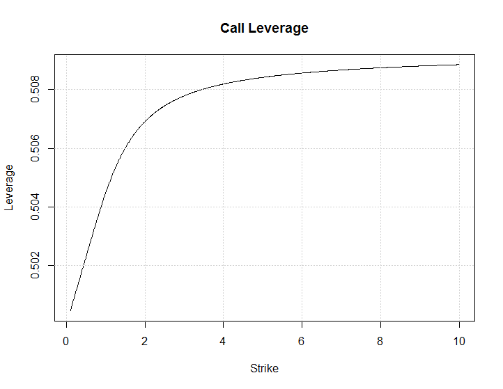
Ciao, I'm studying this problem from a while. Let me post the graph obtained numerically. I've used the following parameters:

$$ \left\{ \begin{array}{rcl} S &=& 2 \\ r &=& 0.01 \\ \sigma &=& 0.2 \\ K &\in& [0.1, 10] \\ T &=& 5 \\ t &=& 1 \end{array} \right. $$

This is not good since the function is always increasing and that means that it has no max value wrt $K$.

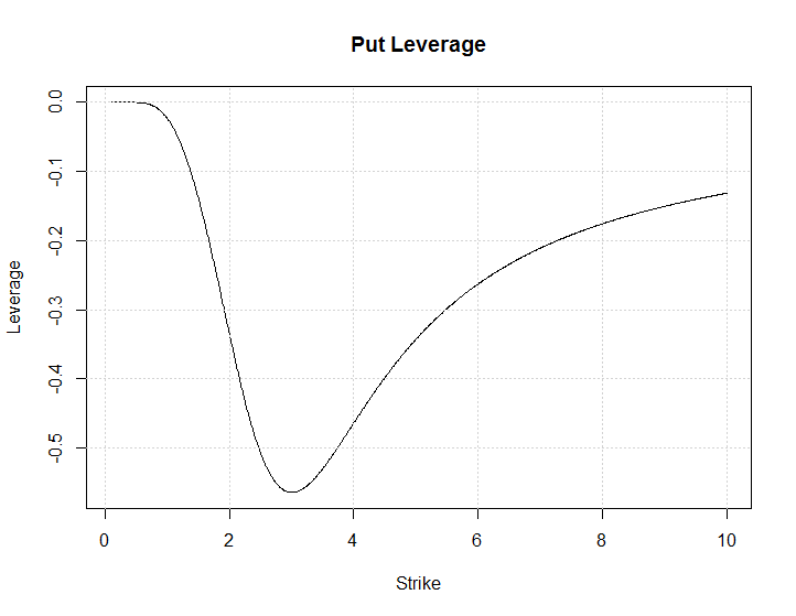
The Put case is really intersting, let me report the plot:

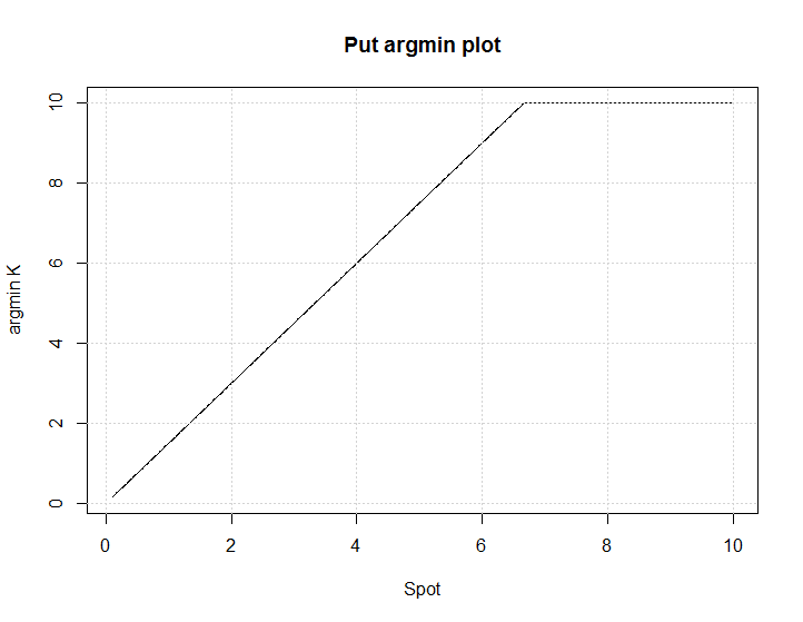
Of course in this case we have a minimum (working very hard for a closed form...in coming). I solved the minimum problem numerically again (in the Put case). In order to do it I've studied the behaviour of the minimum value of $K$ wrt $S$. In turns out that the following equation hold: $$ K_{min} = \frac{3}{2}S $$

This is the R code I've used:

d1 <- function(S, K, sigma, r, T, t){
  return(1/(sigma*sqrt(T-t))*(log(S/K) + (r + sigma^2/2)*(T-t)))
}

d2 <- function(S, K, sigma,r,  T, t){
  return(d1(S, K, sigma, r, T, t) - sigma*sqrt(T-t) )
}

Call <- function(S, K, sigma,r,  T, t){
  return(pnorm(d1(S, K, sigma, r, T, t))*S - pnorm(d2(S, K, sigma, r, T, t))*K*exp(-(T-t)) )
}

DeltaCall <- function(S, K, sigma, r, T, t){
  return(pnorm(d1(S, K, sigma, r, T, t)))
}


Put <- function(S, K, sigma, r, T, t){
  return(K*exp(-r*(T-t)) - S + Call(S, K, sigma, r, T, t))
}

DeltaPut <- function(S, K, sigma, r, T, t){
  return(DeltaCall(S, K, sigma, r, T, t) - 1)
}

leverageCall <- function(S, K, sigma, r, T, t){
  return(DeltaCall(S, K, sigma, r, T, t)/Call(S, K, sigma, r, T, t))
}

leveragePut <- function(S, K, sigma, r, T, t){
  return(DeltaPut(S, K, sigma, r, T, t)/Put(S, K, sigma, r, T, t))
}


minLPut <- function(S, K, sigma, r, T, t){
  LPut = leveragePut(S, K, sigma, r, T, t)
  return(min(LPut))
}

argminLput <- function(S, K, sigma, r, T, t){
  LPut = leveragePut(S, K, sigma, r, T, t)
  return(K[LPut == min(LPut)])
}



S = 2
r = 0.01
sigma = .2
T  = 5
t = 1
K = seq(0.1, 10, by = 0.01)

LCall = leverageCall(S, K, sigma, r, T, t)
LPut = leveragePut(S, K, sigma, r, T, t)

argminLput(S, K, sigma, r, T, t)
argminLput(4, K, sigma, r, T, t)

plot(K, LCall,
     xlab = "Strike",
     ylab = "Leverage",
     type = "l",
     main = "Call Leverage")
grid()

plot(K, LPut,
     xlab = "Strike",
     ylab = "Leverage",
     type = "l",
     main = "Put Leverage")
grid()



S = seq(0.1, 10, by = 0.01)
yS = S
for(i in 1:length(S)){
  yS[i] = argminLput(S[i], K, sigma, r, T, t)
}

plot(S, yS,
     type = "l",
     xlab = "Spot",
     ylab = "argmin K",
     main = "Put argmin plot")
grid()