2
$\begingroup$

I am doing a research exercise where I have two price series $X_t, Y_t$ which I regress against each other and test for cointegration.
Once I confirm that they are cointegrated (using CADF or Johansen test) I derive the equation for the spread as
$$spread_t = Y_t - (\alpha + \beta X_t)$$

or alternatively
$$spread_t = Y_t - \beta X_t$$

where $\alpha$ is the intercept and $\beta$ is the slope coefficient from the regression of $Y_t$ on $X_t$.

As a next step I want to do Monte Carlo simulations to test the simple trading rule.

  • if spread above 2 st.dev wrt equilibrium buy X and sell Y;
  • if spread below 2 st.dev wrt equilibrium sell X and buy Y;

but don't know how to construct the Monte Carlo paths for the simulation.

Could anybody explain how the simulation could be carried out?

Most of the textbooks and research papers explain just how to find asset pairs and test them for the cointegration. Some explain the back-testing on the historical data. I haven't found any explanations how the Monte Carlo simulation could be used to test such trading strategy.

Should be only the spread modeled in the AR(1) like process? It seems that one would need to simulate the asset prices anyway. Should I maybe use the Vector Auto-regressive Model (VAR)? My understanding here is that this would give me some equation again where the spread would be expressed in therms of lagged asset prices.
Each of the two assets doesn't have to be mean reverting. If I model the prices independently how then the relation (cointegration) between them would be preserved?

$\endgroup$
2
  • $\begingroup$ I suppose you meant to regress $Y_t$ on $X_t$ although you wrote (X~Y). $\endgroup$ Commented Sep 4, 2016 at 8:29
  • $\begingroup$ yes I meant the regression $Y_t$ on $X_t$ and alternatively the spread could be without the intercept $spread_t = Y_t - \beta X_t$ $\endgroup$
    – Michal
    Commented Sep 4, 2016 at 18:00

3 Answers 3

1
+50
$\begingroup$

I am somewhat missing the objectivity or the distinctness of the objective of the question. Nevertheless, here are the conclusions on what I have understood.

STEP I: Define and ascertain the minimum number of the data-points you need, for determination of $\alpha$ and $\beta$ and let this minimum number be called as a CHUNK or QUANTUM or BUNDLE. Also define the incremental stepping size e.g. $\mathscr{step\_size}$, by which the chunk would move forward in time. For a $\mathscr{chunk\_size}$ = 1000 and $\mathscr{step\_size}$ = 200, the input data moves from 0 to 1000; 200 to 1200; 400 to 1400; 600 to 1600 and likewise, and let's call these SEGMENTS.

STEP II: Each SEGMENT (after testing for the cointegration), would give somewhat different values for the $\alpha$ and $\beta$ which would give different values for $\mathscr{spread_t}$ form a set of random numbers, though a very closely seeded one. From these SEGMENT values, the decision making can be done.

Note 1: I think it is the first step for which you wish to create MonteCarlo paths for the simulations. With C++, it can be accomplished using OpenMP, though it is quite stone-age primitive for something like MonteCarlo but with some clever tricks, it usually acquiesces to programmer's wishes. Note 2: The crux of the approach is keeping the $\mathscr{step\_size}$ sufficiently short; through which a lot of closely-spaced and random(which is a paradox; hence quasi-random) values for $\mathscr{spread_t}$ can be generated. Note 3: MonteCarlo simulations are fundamentally used where the parametric form of the conditioning has been already established and a large number of experiments needed to be done to ascertain the value of the desired variable. In this case, it can be adjudicated that the parametric form for determining $\mathscr{spread_t}$ has been ascertained and hence a MonteCarlo procedure can be carried out, with introduction of stochastic non-linear weight function in the $\mathscr{spread_t}$ (see below). Please note that, these $\mathscr{chunk\_size}$ and $\mathscr{step\_size}$ themselves can be made random, which would perhaps require more number of experiments to conduct.

Given this problem, my personal approach would be different, somewhat along the lines of:

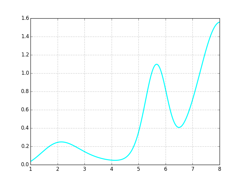
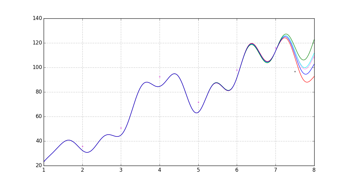
STEP I: Modifying the spread, after the test for the cointegration has been confirmed, as this establishes the linearity of the relationship. Introducing a function such as, $f(t) = k+e^{-\zeta(t, \sigma(t), \eta(t), \delta, \gamma, \cdots)}$, where $k$ is a real number, the shift factor, $\delta$ is a function that gives random number between 0 and 1, accounting for the normalized market-noise (this function mimics the so-called $\epsilon_i$, the random component, in regression analysis) and where $\eta(t)$ is simply the causal function. I would introduce another multiplicative variable $\gamma$ depending upon the historical weights and major share-holders' quantifiable decision making patterns. (It would be much easier, if the $X_t$ and $Y_t$ are the components of the DOW or S&P 500, as the major shareholding figures and the information about shareholders themselves, are easily available for such companies). Please notice that I am deliberately introducing the controlled non-linearity in this relationship for dynamic evaluation of $\mathscr{spread_t}$. Here I have constructed a function for $\eta(t)$ for the NASDAQ:AAPL with only 8 data points, though it is extremely primitive, it does illustrate the way and future trend for the equity in the neighborhood of AUG.19.2016. $$\eta(\tau) = \sin \left( 0.04545\tau \right) \times e^{1.22\sin \tau + \cos \tau} - 0.00840 \times \sin ({\tau}) \times \mathscr{e} ^{-\tau \sin(\tau)}$$ I have used $\tau$ for time-variable for visual clarity in equation.

Given below is a shifted-variation of this as $\eta(\tau-0.77)$ shifted-variation as $\eta(\tau-0.77)$ and here is the final output(though it is very crude due to lack of HP Computing, so the pin-pointing the exact timing is not very reliable. the red line indicates the most probable behavior in the neighborhood of AUG.19.2016, note that the shareholders' quantifiable input has been excluded.
STEP II: Now, from here, I could go on and follow the above standard procedure, with writing OpenMP loops in C++ to conduct as many possible iterations as I could, without getting the cores hanged, to get a lock on the $\mathscr{spread\_t}$. And once, a lock in the predefined trading bandwidth is accomplished, the automated trading can be performed, as per the desired conditions.

Note 1 The idea of cointegration in pairs-trading (and in various other stochastic binary-system analysis/estimate procedures) is basically derived from the fact that, in the long run, the assets, or, in general, the cointegrated pair of variables, usually stabilize toward their equilibrium(or the mean regression); the so-called "long-run-equilibrium"(please note that this is just an informal analogy). And now, the MonteCarlo simulations, work backwards, that is, from the volume or the space of all possible outcomes, and interpreting this volume or the space as the probability; though the analysis and the usual pedagogy of Monte Carlo usually goes to show the equivalence of a Monte Carlo estimate to the Expected value of all possible outcomes for a given well-defined and distinct condition(invoking subsequently the "law of large numbers") and from thereon the usual statistical analysis takes charge. This explains the difficulty in finding Monte Carlo simulation for pairs-trading strategy.

I haven't found any explanations how the Monte Carlo simulation could be used to test such trading strategy.

Also, since the cointegration, establishes a linear relationship between two random walks and Monte Carlo simulations generally don't work well with systems with a linear model. This is why I have introduced a transcedental non-linearity in my approach. Nevertheless, there has been some progress, please see this link. Now, to answer your first question, in theory it is possible to model an asset in isolation (without cointegration and the regressive features, dynamic or otherwise, and various other dependent-variable statistical tools, just using the time-series properties cleverly) but this doesn't generate realistic results. I had used, NASDAQ Composite and NASDAQ:AAPL in the first example. And to answer the second question, in my opinion, it is more of a choice between preserving linearity established by cointegration tests and the realistic results in estimation of future prices. I chose the latter, as it is evident in my approach. Please note that I haven't seen any Monte Carlo simulations for a linear binary system, as of yet. And I could be very well wrong.

Note 2 For a parametric form of relationship which is linear, and its constants of proportionality, whose determination is a key issue in all types of simulation, when forced to a MonteCarlo simulation, requires at least the relation to be dependent not trivially on the non-stochastic terms and functions, for it limits the paths of simulations for such a procedure and yields unnecessary time and memory complexities. Any attempt to force genuine MonteCarlo eradicates the linearity of base relationship. The various methods presented to simulate Cointegrated Systems seem to be good, and can be programmed, in their original form, without invoking MonteCarlo method to get the desired outputs.

$\endgroup$
6
  • $\begingroup$ if I understood correctly you would model each asset separately (or just one asset?) how would be the cointegration implied by historical relation reflected in the simulation? $\endgroup$
    – Michal
    Commented Sep 9, 2016 at 20:25
  • $\begingroup$ I have added a note in the answer. Hope this helps! Cheers! $\endgroup$
    – Madhur
    Commented Sep 10, 2016 at 13:30
  • $\begingroup$ I have found a general example how this could be simulated but I don't know how how could it be linked to historical data $$y_{1t}=β_2 \ \mathbf{y_{2t}} + u_t, \quad \quad where \ \ \ u_t∼I(0) \quad \quad (12.4)$$ $$\mathbf{y_{2t}}=y_{2t-1}+vt, \quad \quad where \ \ \ v_t∼I(0) \quad \quad (12.5)$$ faculty.washington.edu/ezivot/econ584/notes/cointegration.pdf p.435 $\endgroup$
    – Michal
    Commented Sep 10, 2016 at 14:10
  • $\begingroup$ I've searched the pdf for Monte Carlo but I couldn't find any. This is 50 pages long. Can you pinpoint the section or page number where the possibility of simulation has been hinted or given? $\endgroup$
    – Madhur
    Commented Sep 10, 2016 at 15:48
  • 1
    $\begingroup$ Simulation using Phillips triangular representation and Monte Carlo simulation paths are very different things. The former uses additional linearity in a binary base class (notice $\mathbb{I(0)}$ to generate $\mathbb{I(1)}$) to derive the constitutional elements of the $\mathscr{spread_t}$ and the latter relies very heavily on (preferably) multidimensional random walks, in a reverse-way of the usual statistics. I have also found this new method for simulation . $\endgroup$
    – Madhur
    Commented Sep 10, 2016 at 20:02
1
$\begingroup$

You can't use Monte Carlo simulation to test a trading strategy. The parameters (assumptions) you put in the simulation paths will either confirm or reject your hypothesis.

You can't have an agnostic Monte Carlo test. If you do a stochastic test and write out the code for it, you wouldn't need to run it to know what the results would be. Either X and Y are assumed to converge or they aren't. If they converge, the test will yield positive results. If they don't, your portfolio sucks. That's it. If your simulation paths include a rule to converge at z standard deviations, then the portfolio rules will work. If they don't have any rules to converge, then your portfolio rules will suck.

That is why they use historical data. Historical data does not require you to impose any assumptions on the simulation. Either they converge past 2 SD or they don't, but you don't know. You run the test to find out if two securities are cointegrated enough to run a stat arb trading strategy on them successfully.

$\endgroup$
3
  • $\begingroup$ I see your point, but at the same time I don’t think the statement that you can’t test a trading strategy using MC is entirely correct. Once one confirms a specific behavior (in the past) by statistical tests then couldn’t one assume that this behavior would be present in the near future and model Monte Carlo sim under this assumption and then apply and test the trading rules? (after all the investment strategies usually assume that the past is repeatable). $\endgroup$
    – Michal
    Commented Sep 9, 2016 at 20:26
  • 1
    $\begingroup$ You could do a MC sim if you want to test your risk mitigation techniques. If you confirm your trading strategy works with historical data, you can't "further confirm" it using MC sim. MC sim outputs what you input. You should know the expected result of MC sim before you even run it. The reason you use MC sim is you look at your expected losses max losses with VaR using different strategies, then decide which strategy has the most acceptable risk profile.. $\endgroup$
    – milkmotel
    Commented Sep 11, 2016 at 16:54
  • $\begingroup$ to test the risk profiles of the strategies would be the intention of such exercise indeed. The question is then how to build such simulation so that it would be linked to the historical data (link in the sens of price levels, the simulation would start from the last available historical price levels)? $\endgroup$
    – Michal
    Commented Sep 11, 2016 at 18:51
0
$\begingroup$

I think you may confuse with Monte Carlo and time series models you are using. As you said some papers show back test of pair trading strategy, in practice it will do it. After fitting the spread series in in-sample data set (of cause co-integration test valid as well) then optimize parameters, like the trading threshold and stop-loss, then put this strategy in out-sample data set to do the testing. If it performs good and stable, then it's a OK strategy ready to use.

For the Monte Carlo part it's hard to say how you can use directly. In general, you fit the two series Xs & Ys(depends what process you use, usually stocks use lognormal process, then run Monte Carlo to produce sort of "out-sample" data, then fit the spread series on the simulated series, after that do your best to find parameters(too much) that makes a strategy (usually find good parameters around simulation means, and control losses when extremes happen).

$\endgroup$

Your Answer

By clicking “Post Your Answer”, you agree to our terms of service and acknowledge you have read our privacy policy.

Not the answer you're looking for? Browse other questions tagged or ask your own question.