Pricing
In order to answer you question regarding the computation of the delta, I need to take a brief detour into pricing first. When the underlying asset follows a geometric Brownian motion, then barrier options can be easily priced using the method of images; see e.g. Buchen (2001). The notation I use is very similar to the one in my paper Zhang and Thul (2017) and I refer to its appendix A and B for details (sorry for the plug).
Using this approach, we can show that the price of a down-and-out call option with a barrier above the strike is given by
\begin{equation}
\tilde{V}(S, \tau) = \mathcal{A}_B^+(S, \tau) - K \mathcal{B}_B^+(S, \tau) - \stackrel{B}{\mathcal{I}} \left\{ \mathcal{A}_B^+(S, \tau) - K \mathcal{B}_B^+(S, \tau) \right\},
\end{equation}
where
\begin{eqnarray}
\mathcal{A}_\xi^s (S, \tau) & = & S e^{-\delta \tau} \mathcal{N} \left( s d_1 \right),\\
\mathcal{B}_\xi^s (S, \tau) & = & e^{-r \tau} \mathcal{N} \left( s d_0 \right),\\
d_\eta & = & \frac{1}{\sigma \sqrt{\tau}} \left( \ln \left( \frac{S}{\xi} \right) + \left( r - \delta + \left( \eta - \frac{1}{2} \right) \sigma^2 \right) \tau \right),\\
\stackrel{B}{\mathcal{I}} \left\{ \tilde{V}(S, \tau) \right\} & = & \left( \frac{S}{B} \right)^{2 \alpha} \tilde{V} \left( \frac{B^2}{S}, \tau \right),\\
\alpha & = & \frac{1}{2} - \frac{r - \delta}{\sigma^2}.
\end{eqnarray}
Here, $\mathcal{A}_\xi^s(S, \tau)$ if the valuation function of an asset binary option that pays off one unit of the underlying asset if $s S_T > s \xi$ where $s \in \{ -1, +1 \}$ indicates a put or call. Similarly, $\mathcal{B}_\xi^s(S, \tau)$ is the valuation function of a bond binary option that pays off one currency unit. $\stackrel{B}{\mathcal{I}}$ is called the image operator.
To get the derivatives, we use that
\begin{eqnarray}
\frac{\partial}{\partial S} \mathcal{A}_\xi^s(S, \tau) & = & e^{-\delta \tau} \mathcal{N} \left( s d_1 \right) + s S e^{-\delta \tau} \mathcal{N}' \left( s d_1 \right) \frac{\partial d_1}{\partial S},\\
\frac{\partial}{\partial S} \mathcal{B}_\xi^s(S, \tau) & = & s e^{-r \tau} \mathcal{N}' \left( s d_0 \right) \frac{\partial d_0}{\partial S},\\
\frac{\partial}{\partial S} d_\eta & = & \frac{1}{S \sigma \sqrt{\tau}},\\
\frac{\partial}{\partial S} \stackrel{B}{\mathcal{I}} \left\{ \tilde{V}(S, \tau) \right\} & = & \left( \frac{S}{B} \right)^{2 \alpha} \left( \frac{2 \alpha}{S} \tilde{V} \left( \frac{B^2}{S}, \tau \right) - \frac{B^2}{S^2} \frac{\partial \tilde{V}}{\partial S} \left( \frac{B^2}{S}, \tau \right) \right).
\end{eqnarray}
I did not go through the tedious task of checking if this actually agrees with the formula that you referenced.
Code
import numpy
import scipy.stats as stats

def assetBinary1D(maturity, xi, phi, spot, rate, dividend, volatility):
    totalVolatility = volatility * numpy.sqrt(maturity)
    dPlus = (numpy.log(spot / xi) + (rate - dividend + 0.5 * volatility**2) * maturity) / totalVolatility
    dPlusCDF = stats.norm.cdf(phi * dPlus)
    discountFactorDividend = numpy.exp(-dividend * maturity)
    value = spot * discountFactorDividend * dPlusCDF
    derivative = discountFactorDividend * (dPlusCDF + phi * spot * stats.norm.pdf(phi * dPlus) / (spot * totalVolatility))
    return (value, derivative)

def bondBinary1D(maturity, xi, phi, spot, rate, dividend, volatility):
    totalVolatility = volatility * numpy.sqrt(maturity)
    dMinus = (numpy.log(spot / xi) + (rate - dividend - 0.5 * volatility**2) * maturity) / totalVolatility
    discountFactorRate = numpy.exp(-rate * maturity)
    value = discountFactorRate * stats.norm.cdf(phi * dMinus)
    derivative = phi * discountFactorRate * stats.norm.pdf(phi * dMinus) / (spot * totalVolatility)
    return (value, derivative);

def imageOperator(valueFunction, barrier, spot, rate, dividend, volatility):
    alpha = 0.5 - (rate - dividend) / volatility**2
    imageFactor = (spot / barrier)**(2.0 * alpha)
    value, derivative = valueFunction(barrier**2 / spot)
    value2 = imageFactor * value
    derivative2 = imageFactor * (2.0 * alpha / spot * value - (barrier / spot)**2 * derivative)
    return (value2, derivative2)

# attention: only for barriers above the strike!
def downAndOutCall(maturity, strike, barrier, spot, rate, dividend, volatility):
    def valueFunction(spot):
        value, derivative = assetBinary1D(maturity, barrier, 1.0, spot, rate, dividend, volatility)
        value2, derivative2 = bondBinary1D(maturity, barrier, 1.0, spot, rate, dividend, volatility)
        return (value - strike * value2, derivative - strike * derivative2)
    value, derivative = valueFunction(spot)
    value2, derivative2 = imageOperator(valueFunction, barrier, spot, rate, dividend, volatility)
    return (value - value2, derivative - derivative2)
This yields
downAndOutCall(0.2, 1300.0, 1350.0, 1400.0, 0.0, 0.0, 0.2)
>> (65.16660154600855, 1.2863311571074099)
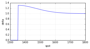
Delta

The delta is, just like the slope of the payoff function, non-negative everywhere.
Edit
Full source code can be found on GitHub.
References
Buchen, Peter W. (2001) "Image Options and the Road to Barriers," Risk Magazine, Vol. 14, No. 9, pp. 127-130
Zhang, Ally Quan and Matthias Thul (2017) "How Much is the Gap? Efficient Jump-Risk Adjusted Valuation of Leverage Certificates," Quantitative Finance, forthcoming, available on SSRN

