8
$\begingroup$

From the formula of the delta of a call option, i.e. $N(d1)$, where $d_1 = \frac{\mathrm{ln}\frac{S(t)}{K} + (r + 0.5\sigma^2)(T-t)}{\sigma\sqrt{T-t}}$, the delta of an ATM spot call option is slightly bigger than 0.5. However, this is unintuitive to me... can anyone explain why?

Also, is there any way to interpret what does $d_1$, and $d_2$ represent where $d_1$ is shown above and $d_2 = d_1 - \sigma\sqrt{T-t}$

$\endgroup$
2
  • $\begingroup$ Did you have look at: en.wikipedia.org/wiki/Black%E2%80%93Scholes#Interpretation? $\endgroup$
    – Bob Jansen
    Commented Nov 23, 2012 at 16:16
  • $\begingroup$ Did you compute the delta numerically or did you use a close form solution ? Can you provide the details of your computation. Did you try to compute your delta with $r=0$ ? Is it simply because of the discounting on the strike ? $\endgroup$
    – BlueTrin
    Commented Nov 23, 2012 at 16:44

4 Answers 4

10
$\begingroup$

The reason you find it counter intuitive is that because you think of it as the probability of ending in the money at the maturity which is not exactly right. Even with a interest rate of $0\%$ where the stock has no tendency to rise or fall you see that delta is slightly higher than $0.5$ for calls ( $\Delta = \sigma * \sqrt T$ ) and here is the reason:

Think of delta as number of shares to hedge. Even when $r=0\%$ because the stock moves with a geometric brownian motion higher stock prices have larger movements so in order to hedge against a call you need more shares than hedging against a put.

Alternatively, for dual delta which is the probablity of ending in the money you see that for at the money options where $r=0\%$ dual delta is $0.5$

$\endgroup$
1
  • 3
    $\begingroup$ Using r=0 is a great simplification that shows the real "culprit" behind the greater than 0.5 delta. $\endgroup$ Commented Nov 24, 2012 at 15:31
8
$\begingroup$

In the no-arbitrage pricing the log return of the stock price does not have expected return $0$ but $r$, the risk free rate. This is strongly related to the pricing of forward contracts. There you could follow the steps to see that in the arbitrage free world the spot price grows with the risk-free rate in expectation.

Thus if you price an option then the probability (in the martingale measure) that the log return is positive is greater than $1/2$ if there are positive interest rates. If you calculate with a dividend yield then this yield is substracted from the risk-free rate.

All the things that I have said hold for the log-return. If you take the exponential: $$ S_0 \exp( X_t ) = S_0 (1 + X_t + \frac12 X_t^2 + \cdots) $$ where $X_t$ is the log return process, and take the expectation then you get the terms $E[X_t] = r t$ for $E[X_t^2]/2 = t \sigma^2/2$ considering terms up to $2nd$ order.

In the Bachelier model, where the stock price is modelled as arithmetic Brownian motion, there you don't have this $\sigma^2$ term.

$\endgroup$
3
$\begingroup$

$N(d_2)$ is the probability of expiring ITM.

$S N(d_1)$, on the other hand, is the conditional expectation of the stock price, where the condition is being above the strike at expiry.

The difference between $d_2$ and $d_1$ accounts for that and arises from the payout equation $\max(S_T-K,0)$, where the expectation of the price at expiry, $S_T = s_0 e^{(r - 0.5*σ²)T}$. When one goes to evaluate the integral $S_T ∫ n(d_1) - K ∫ n(d_2)$, where n(x) = the normal density function $e^{-x²/2} / \sqrt{2π}$, the e terms from $S_T$ and the normal density interact, leading to $d_1$ being higher than $d_2$ to account for conditional expectation.

$\endgroup$
0
0
$\begingroup$

With dividends, $$d1 = ( log(S/K) + (r - d + 1/2*σ^2)*t ) / (σ*sqrt(t))$$ which is identical to $$d1 = ( log(F/K) + 1/2*σ^2*t ) / (σ*sqrt(t))$$ because the forward is computed $F = S e^{(r-q)T}$

Using this, setting $r = d = 0$ will result in delta being > 0.5 for any time $t$ and implied vol $\sigma$ that is > 0 (hence all the time). This comes from the fact that if $d1 =( log(F/K) + 0.5*σ^2*t ) / (σ*sqrt(t))$, you can see that for 100% moneyness, hence $F=K$, $d1>0$ which means it is above 50D which corresponds to N(0.0). It is an increasing function of vol:
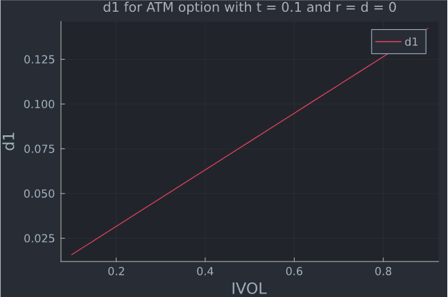
enter image description here

and the term $$\frac{log(\frac{F}{K})}{\sigma\sqrt t}$$ in d1 converges to 0 as $t \rightarrow \infty$ (the larger vol, the quicker it converges), which leaves us with $1/2∗σ2∗t$ which in turn is growing withough bound in $t$ and $\sigma$.
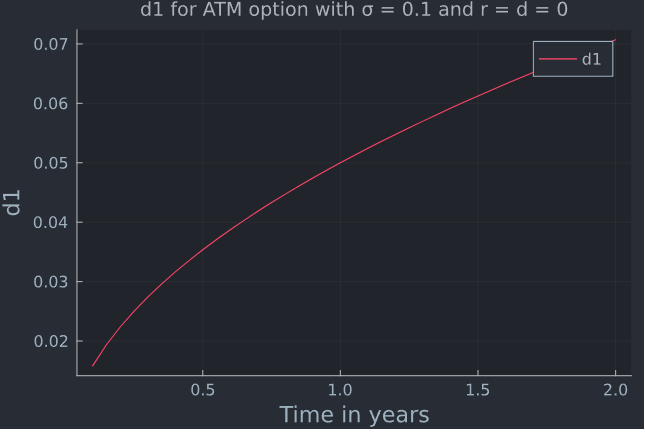
enter image description here

With interest rate and dividends, it depends on the forward, just like @Richi W explained. In the following App I made in Julia, I price an ATM option, with 365 days to maturity, and an IVOL of 10%. The horizontal axes shows different interest rates, and dividends are set to 0. The vertical line shows the zero interest case and on the horizontal line corresponds to 0.5 delta. You can clearly see how different interest rates affect delta for an ATM option.
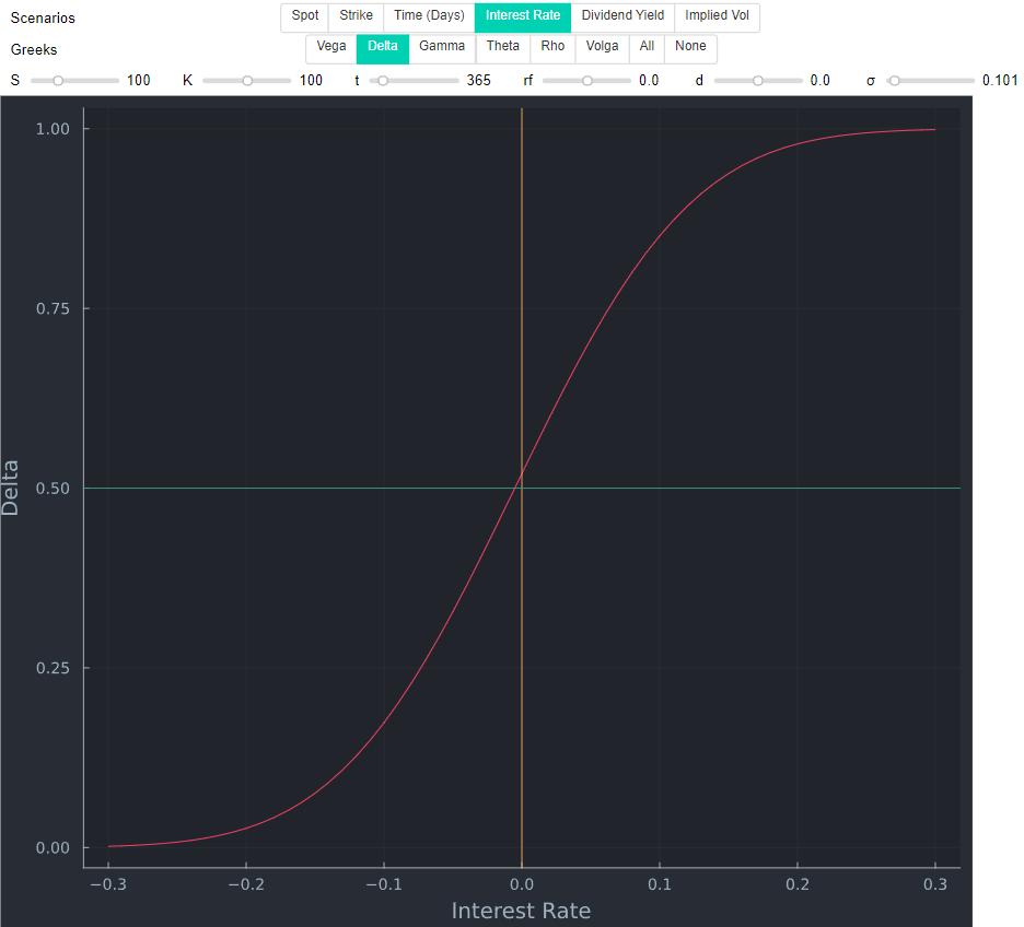
enter image description here

The same (in opposite direction) is true for different dividends (for convenience, rates are set to 0).
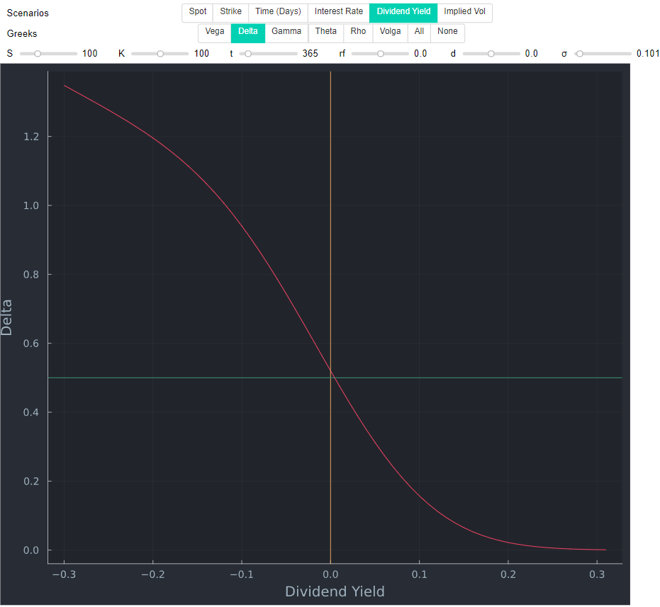
enter image description here

Last but not least, the risk-adjusted probability of the event that the option will finish in the money is P(ST>X)=N(d2), as shown in Understanding N(d1) and N(d2): Risk-Adjusted Probabilities in the Black-Scholes Model by Lars Tyge Nielsen for example. Contrary to another answer, this is also not a constant of 0.5 for ATM options but tends to 0 if $t \rightarrow \infty$ and / or $\sigma \rightarrow \infty$ as shown in this answer.

$\endgroup$

Your Answer

By clicking “Post Your Answer”, you agree to our terms of service and acknowledge you have read our privacy policy.

Not the answer you're looking for? Browse other questions tagged or ask your own question.