Max allowable return in Markowitz model

Question

The Markowitz model solves the following problem: The portfolio with the smallest variance among attainable portfolios with expected return µV.

Here we have to choose µV to get the optimal portfolio weights.

My question is: What are the bounds on the values that µV can take? In particular, what is the maximum possible attainable return µV?

Answer 1

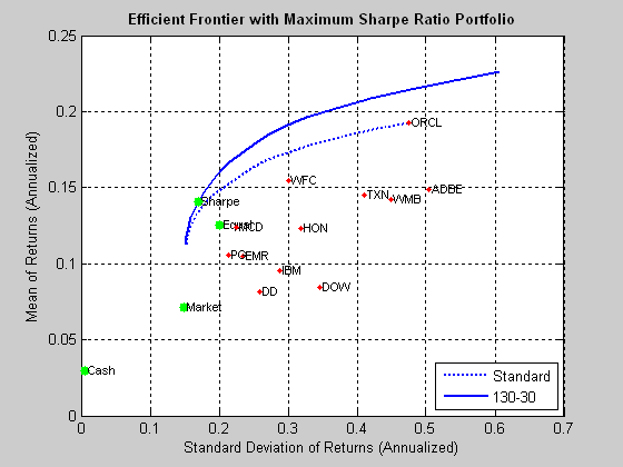
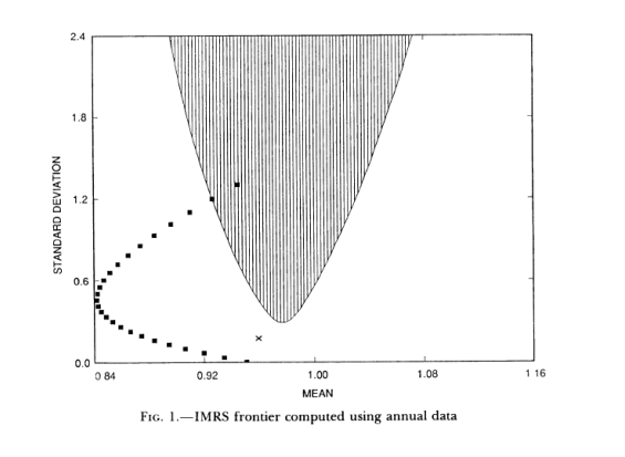
The Markowitz mean-variance model takes in some target expected portfolio return $\mu_T$ as an input and returns optimal portfolio weights $\boldsymbol\omega$ that minimize risk for that return. Repeating this for a series of target returns, $\boldsymbol\mu_T$, manifests two different efficient frontier curves (series of efficient portfolios) depending on the investment scenario:

1. Unconstrained efficient frontier (short-selling allowed), thick line
2. Constrained efficient frontier (short-selling forbidden), dotted line

The optimization problem for the unconstrained efficient frontier (1) is: \begin{equation} \begin{aligned}[l] \hat{\boldsymbol{\omega}}(\mu_T) = &\min_{\boldsymbol{\omega}} \boldsymbol{\omega}^{\top} \hat{\mathbf{\Sigma}} \boldsymbol{\omega} & \\ s.t. \enspace & \boldsymbol{\omega}^{\top}\boldsymbol{\mu} = \mu_T\\ & \boldsymbol{\omega}^{\top}\boldsymbol{\iota}_N = 1 & \\ \end{aligned} \end{equation}

The optimization problem for the constrained efficient frontier (2) is: \begin{equation} \begin{aligned}[l] \hat{\boldsymbol{\omega}}(\mu_T) = &\min_{\boldsymbol{\omega}} \boldsymbol{\omega}^{\top} \hat{\mathbf{\Sigma}} \boldsymbol{\omega} & \\ s.t. \enspace & \boldsymbol{\omega}^{\top}\boldsymbol{\mu} = \mu_T\\ & \boldsymbol{\omega}^{\top}\boldsymbol{\iota}_N = 1 & \\ & \omega_n\in \mathbb{R}_{\geq 0}\enspace \forall N & \end{aligned} \end{equation}

The last line shown is the non-negativity constraint for the no short-sales frontier. As long as mean-variance model assumptions are active and standard deviation of each asset is positive, as well as the mean of the asset means vector, $\boldsymbol\mu$, then:

The maximum return on the unconstrained frontier is $\mu=\infty$, although realistically there is a feasible limit to which you would try values for $\mu_T$ to generate a good-enough mean-variance graph, knowing that the unconstrained curve peters out at some level of $\mu$ the higher you go, but still increases at a diminishing rate.

The maximum return on the constrained frontier is max($\boldsymbol\mu$), that is, the expected return of the asset in the investment pool that has the highest expected return. For example, if asset #3 of $N=10$ total assets has an expected return of 5%, you would plug $\mu_T=5\%$ into optimization problem 2 and get back the farthest point, in mean-variance space, where the constrained frontier ends, which is a 100% allocation to the max-return asset (asset #3), or single-asset portfolio. Oracle's stock, shown in the figure, is a separate example that clearly shows the end of the constrained curve.

Normally, neither the unconstrained nor the short-sale constrained efficient frontiers end at the tangency (maximum Sharpe ratio) portfolio, but knowing the location of the tangency on both curves can serve as a guideline as to what cap to place on the highest feasible $\mu_T$ used for tracing the unconstrained frontier (1), knowing that the unconstrained tangency normally has a higher \mu than the constrained tangency. Otherwise, plotting the unconstrained frontier together with the constrained frontier (2) will likely show the constrained one being squashed horizontally relative to the potentially much wider unconstrained one. As for the height of the two frontiers, the unconstrained frontier (1) is normally taller than the constrained frontier (2).

Everything explained so far addresses the upper bound for both frontiers. For the lower bound $\mu_T$ on both, try the global minimum variance (GMV) portfolio that removes the target return constraint. The GMV is a frontier portfolio, but technically is not an efficient portfolio (neither is it an inefficient one):

\begin{equation} \begin{aligned}[l] \hat{\boldsymbol{\omega}}_{GMV} = &\min_{\boldsymbol{\omega}} \boldsymbol{\omega}^{\top} \hat{\mathbf{\Sigma}} \boldsymbol{\omega} & \\ s.t. \enspace & \boldsymbol{\omega}^{\top}\boldsymbol{\iota}_N = 1 & \\ \end{aligned} \end{equation}

Since the inefficient frontier is conceptually an upside-down mirror image of the efficient frontier, you can otherwise try values less than $\mu_{GMV}$ such as the negatives of the upper bound target-returns you decided to use for the efficient frontier: $-\mu_T$.

Answer 2

The maximum attainable return is unbounded as in the model you can borrow without limit. However, what matters in that model is what is the maximum sharpe ratio you can attain.

That has bounds, which are given by the Hansen-Jagannathan distance.

Let me show you what the JH distance looks like. From the law of one price:

\begin{equation} 1 = E [R_{i,t+1} m^\star_{t+1}] \end{equation}

Therefore:

\begin{equation} 1 = E(R_{i,t+1}) E(m^\star_{t+1}) + Corr(R_{i,t+1}, m^\star_{t+1}) Std(R_{i,t+1}) Std(m^\star_{t+1}) \end{equation}

Rewrite the equation above using $R_{f,t+1} = 1/E(m^\star_{t+1})$ to get:

\begin{equation} \frac{E(R_{i,t+1}) - R_{f,t+1}}{Std(R_{i,t+1}) } \leq \frac{Std(m^\star_{t+1})}{E(m^\star_{t+1})} \end{equation}

The left hand side equation is the maximum attainable sharpe ratio. And the equation on the right gives you the bound so: The max Sharpe ratio in the economy is then bounded by the minimum variance SDF volatility over mean!

How do we use these?

• Take $N$ assets. Compute excess returns.
• Estimate variance covariance matrix of returns $\Sigma = E[R R']$ and average payoffs $E(R_{t+1})$. Usually the first one we estimate by taking a large sample and computing covariance matrix and the latter just by averaging returns.
• Plot the above locus and compare with your candidate SDF;

The locus should deliver something like this: