Is Local Volatility a function of the Strike or the Underlying price?

Question

Long story cut short: I am asking why the Local Volatility function can be thought of as a function of the underlying, when in fact it appears to be a function of the strike.

Additionally, I wonder how the local vol process for the underlying, being a single unique process, achieves to generate the same option prices as multiple B-S processes (each with a different constant volatility).

Long story:

The well-known Dupire local volatility formula is:

$$\sigma_{loc}(K,T)^2 =2\frac{\frac{\partial}{\partial T}(C)+rK\frac{\partial}{\partial K}(C)}{K^2\frac{\partial^2}{\partial K^2}(C)}$$

Above, $C$ is the Call option price, and $\sigma_{loc}(K,T)$ is a "local volatility" function which depends on strike and maturity. Let's assume that the underlying is an instrument denoted as $S(t)$, with today's price being $S_0$.

Let's now fix maturity so we only deal with a two-dimensional smile, and let's compute the partial derivatives of the Call option price with respect to strike:

$$C(S_0,T,K,\sigma)=\mathbb{E}^Q\left[(S_T-K)\mathbb{I}_{S_T>K}\right]=\int_{h=K}^{\infty}(h-K)f_{S_T}(h)dh=\\=\int_{-\infty}^{\infty}hf_{S_T}(h)dh-\int_{-\infty}^{h=K}hf_{S_T}(h)dh-\int_{-\infty}^{\infty}Kf_{S_T}(h)dh+\int_{-\infty}^{h=K}Kf_{S_T}(h)dh$$ and taking the derivative: $$\frac{\partial C}{\partial K}=0-Kf_{S_T}(K)-1+\left(\mathbb{P}(S_T<K)+Kf_{S_T}(K)\right)$$ and differentiating again: $$\frac{\partial^2 C}{\partial K^2}=f_{S_T}(K)$$

We see that the partial derivatives of $C$ with respect to $K$ are functions of $K$.

Question: How do these become functions of the underlying?

My thinking is that the strikes are "fixed" and the PDF of the underlying is centerd on $S_0$, so that effectively, $f_{S_T}(K)$ is a function of the distance of $K$ from $S_t$: so as $S_t$ changes (evolves), $f_{S_T}(S_t)$ also changes for every given $K$; is this correct?

Answer 1

The local volatility SDE $$ dS_t = \sigma_{LV}(S_t,t)S_t dW_t $$ is the starting point. (Some absorb the $S_t$ into $\sigma_{LV}(S_t,t)$ but let's keep them separate here).

Starting from this SDE there are two ways to derive the Dupire equation:

1. Using Feynman-Kac theorem to derive the forward Kolmogorov / Fokker-Planck equation from which the Dupire equation follows. This is the most general way, and the route Dupire followed.

2. Using Tanaka's formula and conditioning to show that the Dupire equation is satisfied if local volatility is regarded as a conditional expectation of a stochastic volatilit \begin{align} dS_t &= \sigma_t S_t \left(\rho dW_t + \sqrt{1-\rho^2} dZ_t \right) \\ d\sigma_t &= a(\sigma_t,t) dt + b(\sigma_t,t) dW_t \end{align} where $W$ and $Z$ are independent standard Brownian motions, and $\rho \in (-1,1)$. Because (to be shown shortly) in this case LV is regarded as a conditional expectation of SV, and there are LV functions that cannot be written as a conditional expectation of SV, this is not the most general derivation. But it is useful nevertheless because (I think) it is easier to understand how you get $\sigma_{LV}(K,T)$ when you started out with $\sigma_{LV}(S_t,t)$.

So, proceeding with method 2:

Tanaka's formula is a generalisation of Ito's formula for discontinuous functions. In other words it allows us to write $$ d(S_u - K)_+ = \theta(S_u-K) dS_u + \frac12 \delta(S_u-K) (dS_u)^2 $$ where $\theta$ is the Heaviside function and $\delta$ the Dirac delta function.

Integrating both sides from $t$ to $T$ gives \begin{align} \int_t^T d(S_u - K)_+ &= (S_T-K)_+ - (S_t - K)_+ \\ &= \int_t^T \theta(S_u-K) dS_u + \frac12 \int_t^T \sigma_u^2 S_u^2 \delta (S_u - K) du \end{align}

Now take expectations, and using the fact that $S_t$ is drift less (the generalisation to include $r,q$ is straigtforward), $$ C(S_t,t,K,T) = (S_t - K)_+ + \frac12 \int_t^T E_t \left[ \sigma_u^2 S_u^2 \delta (S_u - K) \right] du $$ where it is assumed the necessary technical conditions are satisfied to take the expectation inside the integral.

Applying conditioning: \begin{align} E_t \left[ \sigma_u^2 S_u^2 \delta (S_u - K) \right] &= E_t \left[ S_u^2 \delta(S_u-K) E_t \left[\left. \sigma_u^2 \right| S_u \right] \right] \\ &= \int_0^\infty x^2 \delta(x-K) E_t \left[ \left.\sigma_u^2 \right| S_u = x \right] q(x,u;S_t,\sigma_t) dx \end{align} where $q(x,u;S_t,\sigma^2_t)$ is the density of $S_u$ (at time $u$) given $\sigma^2_t$ and $S_t$.

The effect of the Dirac delta function is then to single out $x = K$ leading to $$ E_t \left[ \sigma_u^2 S_u^2 \delta (S_u - K) \right] = K^2 q(K,u;S_t,\sigma^2_t) E_t \left[ \left.\sigma_u^2 \right| S_u = K \right] $$ So, $$ C(S_t,t,K,T) = (S_t - K)_+ + \frac12 \int_t^T K^2 q(K,u;S_t,\sigma^2_t) E_t \left[ \left.\sigma_u^2 \right| S_u = K \right] du $$

Now use the fact that (by Breeden-Litzenberger) $$ q(K,u;S_t,\sigma^2_t) = \frac{\partial^2}{\partial K^2} C(S_t,t,K,u) $$ to obtain $$ C(S_t,t,K,T) = (S_t - K)_+ + \frac12 \int_t^T E_t \left[ \left.\sigma_u^2 \right| S_u = K \right] K^2 \frac{\partial^2}{\partial K^2} C(S_t,t,K,u) du $$ The final step is to differentiate both sides wrt the maturity date $T$: $$ \frac{\partial}{\partial T} C(S_t,t,K,T) = \frac12 E_t \left[ \left.\sigma_T^2 \right| S_T = K \right] K^2 \frac{\partial^2}{\partial K^2} C(S_t,t,K,T) $$

This is the Dupire equation with $$ \sigma^2_{LV}(K,T) = E_t \left[ \left.\sigma_T^2 \right| S_T = K \right] $$

Finally then, to answer your first question, what $\sigma^2_{LV}(K,T)$ means is that if at time $T$ the stock takes value $S_T=K$, then the local volatility $\sigma^2_{LV}(S_T,T) = \sigma^2_{LV}(K,T)$. Here $K,T$ are arbitrary in the sense that it is assumed you have options for all strikes and maturity dates. In other words, when valuing exotics, and you need to simulate the stock price and input all possible future values of $\sigma^2_{LV}(S_u = \{K\},u)$, you can find these values from the current observable market prices.

The answer to your second question should now be clear I think.

Answer 2

In addition to the great answer given above, I would like to add an additional perspective by recognizing that my confusion (as per the question) boils down to what is explained in the Derman-Kani paper, which is a "predecessor paper" to the "Local Volatility" paper by Dupire.

In their paper titled "The Volatility Smile and Its Implied Tree" from 1994, Derman and Kani explain how a unique Binomial tree (with time-varying volatilities and implied probabilities) can be extracted from option prices with a smile.

For our simple case here, we just consider two options from the paper and we demonstrate that one unique tree with varying volatility can generate the same two option prices as two different trees with a constant volatility.

We note that in our simple case, the initial price of the underlying is $S_0=100$. The two options we consider are:

• ATM call, $K=100$, 2-year expiry, $IV = \sigma_{BS}=10\%$
• OTM call, $K=110.52$, 2-year expiry, $IV = \sigma_{BS}=9.47\%$

Rates are 3% per year.

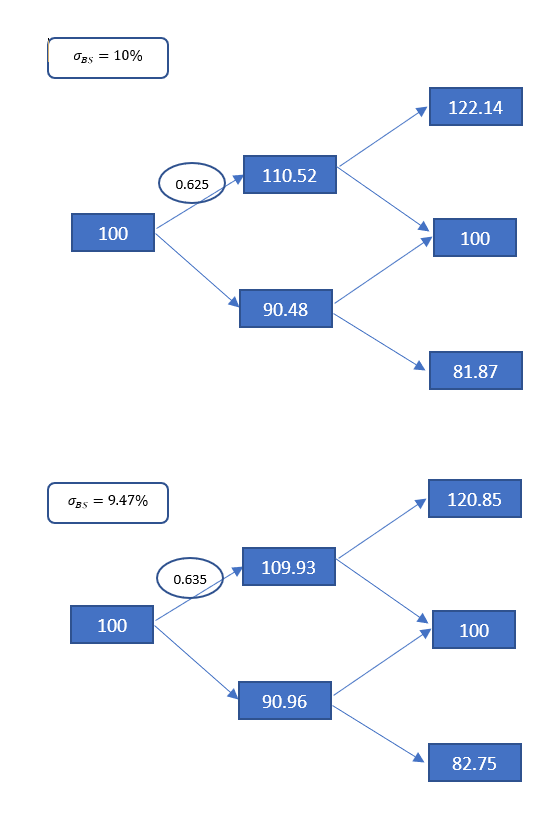
In the B-S world, the two IVs give rise to two different Binomial trees with constant volatilities (the trees are constructed as $S_{t+1}^{up}=S_{t}e^{\sigma_{bs}}$, $S_{t+1}^{down}=S_{t}e^{-\sigma_{bs}}$):

Pricing the two options:

$$C(t=2,K=100,r=0.03,S_0=100,\sigma_{BS}=0.1)=\\=\frac{(122.14-100)*0.625^2}{1.03^2}\approx8.15$$

$$C(t=2,K=110.52,r=0.03,S_0=100,\sigma_{BS}=0.0947)=\\=\frac{(120.85-110.52)*0.635^2}{1.03^2}\approx3.92$$

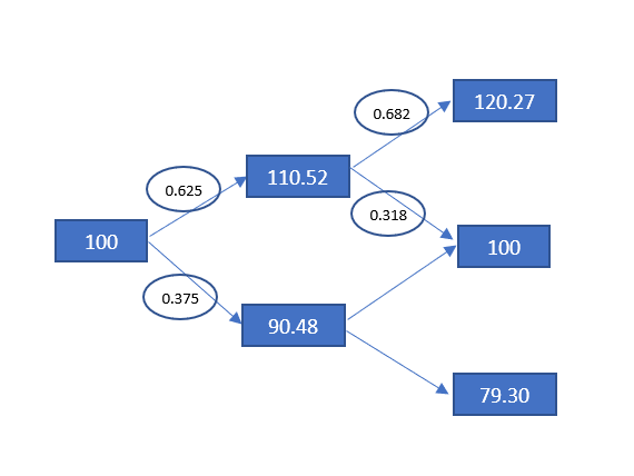
Now, interestingly, Derman & Kani show that a single unique Binomial tree with a varying volatility can be derived from the value of these two option prices (together with imposing a condition that the tree has to recombine).

I skip the derivation of the tree and just show it below:

Again, pricing the two options:

$$C(t=2,K=100,r=0.03,S_0=100,\sigma_{BS}=0.1)=\\=\frac{(120.27-100)*0.625*0.682}{1.03^2}\approx8.14$$

$$C(t=2,K=110.52,r=0.03,S_0=100,\sigma_{BS}=0.0947)=\\=\frac{(120.27-110.52)*0.625*0.682}{1.03^2}\approx3.92$$

So the above construct illustrates that a single unique tree with varying volatility and probabilities can price options with a smile, as opposed to essentially having to use two different trees (processes) corresponding to the two implied vols in the B-S world.

Intuition: Focusing on the unique tree with varying volatility and probabilities, we see that the "implied" volatility in the upper branch between $t_1$ and $t_2$ is $e^{\sigma(t_1,t_2)}=ln\left(\frac{120.27}{110.52}\right)\approx8.45\%$; we can therefore see that the unique implied tree starts off with a volatility of $10\%$ between $t_0$ and $t_1$ but then reduces the volatility in the upper branch to $8.45\%$, whilst "increasing" the implied probability of the up-move from 0.625 to 0.682: in other words, by varying these two parameters (volatility and implied probability), the tree can solve for these two "unknowns" to satisfy the two equations for the two option prices (together with the "anchoring" condition that the tree recombines).

Extrapolating this logic to the local volatility model, which reads:

$$S_t=S_0+\int_{h=t_0}^{h=t}\mu_hS_hdh+\int_{h=t_0}^{h=t}\sigma(S_h,h)S_hdW_h$$

one can intuitively guess that by varying the local volatility function across time and the underlying price, one should be able to recover option prices which correspond to the different constant BS volatilities (i.e. in the tree case, the "local-vol" tree has the feature that the average varying volatility between $t_0$ and $t_2$ is roughly equal the average of the B-S volatilities across strikes for options expiring at $t_2$. So for the continuous case, given a fixed point in time, at an intuitive level, we should have that the average of BS volatilities across all strikes for that given maturity is roughly equal to the time-average of the integral of the local vol function up to that maturity).

As far as the local vol function being a function of strike vs. a function of the underlying, it is now easier to see that the strike appearing the the local vol formula is just a parameter that allows one to extract the required local vol value from the given option prices: once the local vol values had been extracted for all possible values of $K$ across all maturities, it is then just a question of changing the argument of the local vol function from $\sigma(K,t)$ to $\sigma(S_t,t)$ so that the local vol function can be used in the SDE for the evolution of the underlying.