Attribute P&L to PCA vectors (swaps)

Question

I have a daily US swaps data here for 2020 https://easyupload.io/yh4rnd . I have run PCA on standardized data and got PCA matrix (and basic statistics):

I also have such hypothetical portfolio that in this example is making +$195k.

Question: How do I attribute this P&L to each principal component, such that the total P&L number equals +$195k?

Working through suggestion by Dimitri:

Assuming we cannot fully reprice portfolio using a perturbed interest rate curve, so will go with DV01s. To calculate ci for each PCi I converted PCA on standardized data back to unstandardized and calculated weights below for each tenor x PC, then for each PCi I calculated Open and Close in % (eg PC1 opened at 1.94 and closed at 1.89) with c1 euqal to -5.58bp (I checked, each PCi is orthogonal). I then used the same weights to convert original risk from hypothetical book into PCi. I then multiply ciPCi x δ to get P&L. But it doesn't seem to match up, which step am I getting wrong?

Answer 1

Linear PnL is usually correctly estimated by the inner product of risks and market movements::

$$ Pnl = S \cdot \Delta r = S^T \Delta r$$

Where you apply a linear transformation to those risks to express it in some other mathematical basis (e.g. PCA respresentation), then you have some transformation matrix, $T$, and it is easier to show that the PnL is invariant if you perform the following:

$$ \underbrace{T S}_{\text{transformed risk}} \cdot \underbrace{T^{-T} \Delta r}_{\text{transformed changes}} = S^T T^T T^{-T} \Delta r = S^T \Delta r = Pnl$$

Therefore the market movements should be transformed using the inverse-transpose of the original transformation matrix.

Mathematically this is an expression of covariant and contravariant transformations, if you care to investigate further.

Note that you should be able to check your matrix calculations by supplying your portfolio risks such that they align with just on PC (e.g. the first) and ensure that the resulting PCA risks appear to show risk purely to this PC, as in:

Answer 2

Back in the day, I used to do precisely this on a cross-asset basis. The critical point being that the correlations of any of your PCs to any other PC will be zero, else you will have miscalculated your PCs in the first place.

This being a given, you can regress your P&L to any and every PC in isolation, safe in the knowledge that all the others are irrelevant, because they are completely uncorrelated ;-)

Excel's "=SLOPE(y-array,x-array)" will usually suffice. Sometimes, the intercept will create funnies. In which case, "=SUMPRODUCT(y-arrayx-array,x-arrayx-array)" (ie an intercept-less regression) usually works.

hope this helps, DEM

Answer 3

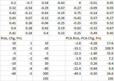
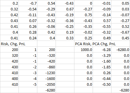
You're right - I've looked, and there are many good tutorials on IR curve PCA out there, e.g. https://mockquant.blogspot.com/2010/12/principal-component-analysis-to-yield.html , https://plus.credit-suisse.com/r/kv66a7 , but I don't see anywhere a good explanation of atributing P&L to the IR curve changes in terms of PCs. Therefore I will outline it. Please ask if any details are unclear and suggest edits if you see errors.

We assume that:

You use the same instruments on day 0 and day 1 to bootstrap the interest rate curve. The interest rate curve is defined by the levels of the instruments.

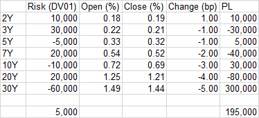
You know the change for each instrument from day 0 to day 1.

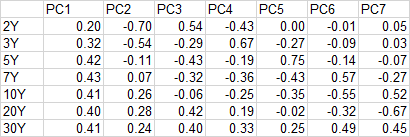
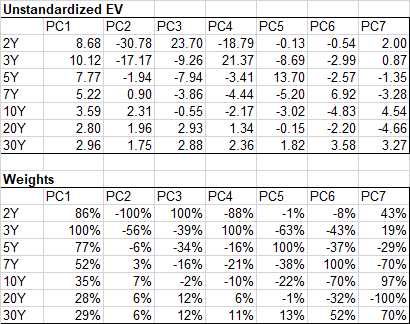
You know the loadings (the weight of each instrument) of the $p$ principal components, denoted $PC_1\ldots PC_p$.

However I don't want to assume that the interest rates sensitivities are strictly linear, i.e. that the dv01's tell us the whole story of the IR risk. Rather, we want the methodology to work even for highly non-linear instruments. You should fully reprice the portfolio using a perturbed interest rate curve if you can. However if you cannot fully reprice, and must estimate the P&L from the dv01's, let $\delta$ denote the vector of dv01's (P&L from small changes in each instrument, interest rate deltas).

Let $Y_0$ denote the interest rate curve on day 0, $M_0$ the mark to market on day 0, and $Y_f$ denote the interest rate curve on day 1.

In order to explain the P&L, we want to explain the change in the interest rate curve levels from $Y_0$ to $Y_1$ in terms of the PC's - each $PC_i$ moved by some $c_i$ that we will find.

For $i=1$ to $p$ - start loop on the principal components

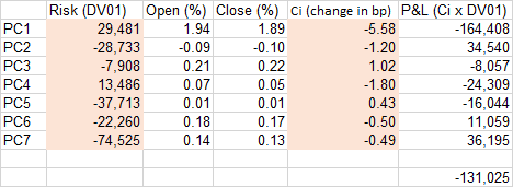
Solve for $c_i$, the change in the interest rates attributable to $PC_i$, that minimizes the distance between $Y_i \stackrel{\mathrm{def}}{=} Y_{i-1} + c_i PC_i$ and $Y_f$.

For better transparency, output $c_i$, and $c_i PC_i$ - the changes in the instruments explained by $PC_i$.

Estimate the P&L contribuion of each instrument by multiplying $\delta$ and $c_i PC_i$. Report these P&L estimates and their sum (the P&L from $PC_i$ move estimates from dv01's).

If you can fully reprice the profolio: let $M_i$ denote the mark to market using curve $Y_i$. Report $M_i - M_{i-1}$ as the more accurate P&L attributable to the $c_i$ change in $PC_i$.

For a more complete picture, if $i>1$, then let $y'_i$ denote $y_0 + c_i PC_i$ - the interest curve obtained by perturbing only $PC_i$ and no other PCs. Reprice the profolio: let $M'_i$ denote the mark to market using curve $Y'_i$. Report $M'_i - M_0$ as the P&L attributable to the $c_i$ change in $PC_i$ and no other PCs.

Otherwise if you don't want to fully reprice, then just use the P&L estimated from the dv01's.

Next $i$ - end loop on the principal components

Report residual P&L not explained by this methodology.