Questions on options cost of carry, and relationship to futures cost of carry

Question

I'm trying to grasp what exactly the effects of higher ongoing interest rates are on holding calls/puts. I am not asking what the effect of a change in interest rates is on call/put prices.

I'm interested chiefly in equity and equity-index options (though I expect the answers are the same for bond futures, replacing dividend yield with coupon yield?).

I understand the cost of carry on equity or equity index futures (I hope) okay. After all, it's pretty easy. Futures price = underlying price + [normalised] interest rate - [normalised expected] dividend yield. So while you carry (long) a future its value decays in line with the interest rate (assuming $r>d$), since the price of the future at expiry converges with the underlying. And obviously a shorted future's value appreciates in line with the interest rate.

Now I also understand (I hope) that one can create a synthetic future using a long ATM call and a short ATM put. I'd be rather surprised if the cost of carry for this synthetic future was any different than for the actual future. So I'd expect that the combined cost of carry of the sold put and the bought call to come to (interest rate - dividend yield) as per a long future position.

What I want to know is how this cost of carry is to be divided between the constituents (long call, short put) of the synthetic future, if one holds one or the other. I assume that it is related to moneyness - that a deep ITM call has cost of carry nearly equal to that of the long future (at which price the deep OTM put has almost zero cost of carry). And that a deep ITM short put also has cost of carry equal to that of the long future (at which price the deep OTM call has almost no cost of carry).

If I were to hazard a guess as to what proportion of the future's cost of carry is payable on a put or call I would guess that it is in proportion to delta (e.g. long put cost of carry = delta * long future's cost of carry, which would be of opposite sign since the delta of the long put is negative). But that's a guess.

Can anyone enlighten me further?

Thanks

Answer 1

Both answers already address the gist of the question. I decided to add (quite) some details because I think there is some confusion from the OP. It is not the future that has carry costs or benefits but the underlying. This is also an important fact for pricing options. However, there is no additional "feature" to the cost of carry that is not already incorporated in the forward pricing if you replicate a forward synthetically. Any deviation from the fair future (zero cost as no one is made better or worse off) will result in a compensation of one counterparty. That's it. The rest below just elaborates on this.

The following screenshot displays for various different implied volatilities (IV), the associated call (c) and put (p) values computed with Black Scholes (with cost of carry), Black76 (without cost of carry but using the forward / future as the underlying), the fair forward / future (Fwd), the strike used, the price of the synthetic long future/forward (C-P), and the compensation for not using the fair forward /future $((F-K)*e^{-r*t})$, as well as the Put & Call values computed with put call parity (PCP). As you can see, forwards and synthetic forwards always match each other in terms of pricing and the cost of carry is always the same. The code and explanations will follow below.

As you can see, all that matters is where K is relative to the fair future. The option prices always adjusts for this and simply resemble the price of the forward /future (as should be, otherwise there would be arbitrage).

Details

The Black Scholes Merton (BSM) and Black 76 option pricing models are both well-known and widely used. The only model difference versus the BSM model is that the underlying future in the Black model has no carry costs or benefits.

In words, the cost of carry relationship describes the relative cost of buying a stock with deferred delivery (the future) versus buying it in the spot market with immediate delivery and "carrying" it forward. If you buy stock now, you tie up your funds and incur a time value of money cost of $r$ per period. On the other hand, you receive dividend payments (carry benefit) of $d$. (Technically, being short spot inverses this and the cost of carry is the cost of paying dividends).

This advantage must be offset by a differential between the futures and the spot price. Therefore, OPs comment made in @Jan Stuller's answer makes no sense:

If it were immaterial everyone would buy ATM calls, sell ATM puts, and sell futures. Net price movement of such a strategy is zero, yet selling futures earns one (interest rate - dividend yield) every year. Which would be free money that I could leverage as high as my broker would let me.

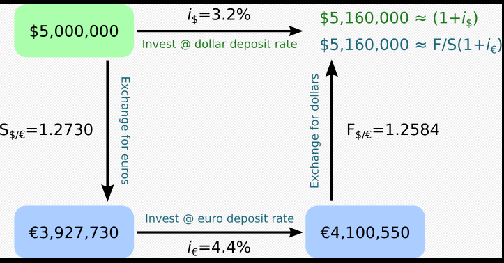
The future price is exactly offsetting this difference and there is no free money. It may be less obvious with equity but should be quite clear with FX (where the concept is identical, just with two interest rates). It is called Covered Interest Parity (CIP).

No matter what you do, returns from investing domestically are equal to the returns from investing abroad. This works because you enter a forward and fix that rate that guarantees no arbitrage.

Now, back to options, let’s begin with BSM which has the carry costs (and benefits) of the underlying incorporated. After all, the model is for European options (hence deferred delivery) just like equity futures, but it has the spot market as the underlying (like equity futures). Writing BSM in Julia looks like this (I like to use it because the code looks almost like a math textbook and the language offers simple, yet powerful plotting libraries paired with speed):

using Distributions
N(x) = cdf(Normal(0,1),x)
function BSM(s,k,t,r,d, σ, cp)
    d1 = ( log(s/k) + (r -d+ σ^2/2)*t ) / (σ*sqrt(t))
    d2 = d1 - σ*sqrt(t) 
    opt = exp(-d*t)*cp*s*N(cp*d1) - cp*k*exp(-r*t)*N(cp*d2)
    delta = cp*exp(-d*t)*N(cp*d1)
    return opt, delta
end

CP is a call put flag (1 for call, -1 for put). Ignoring it, one has the following formula:

$$e^{-d*t}*S*N(d1) - K*e^{-r*t}*N(d2)$$

where $d$ is the dividend, $r$ is the risk-free rate and $d1$, $d2$ are the standard BSM model inputs as shown on Wikipedia. To highlight the carry benefit adjustment in the BSM model, one can rewrite the call and put value as the present value (PV) of the expected option payoff at expiration.

$$E(c_T) = \color{blue}{S*e^{(r-d)*T}}*N(d1) - K*N(d2)$$ and $$E(p_T) = K*N(-d2) - \color{blue}{S*e^{(r-d)*T}}*N(-d1)$$

It should be clear now why the cp flag in the BSM function in the Julia code works.

This also shows nicely that the BSM model value is really just a dynamically managed portfolio of the stock and zero-coupon bonds (the financing part, which can also be seen as bank borrowing or lending). The discounted price of the zero coupon bond is $K*e^{-r*T}$, the stock itself is influenced by the carry benefits (cb) and high cb will lower the call option price. In summary, for calls, one needs to by N(d1) stocks (adjusted for the carry benefit) and N(d2) bonds. Since N(d2) < 0 and N(d1) > 0 one needs to borrow to buy the stock.

Now, let's plug in some hypothetical numbers. I'll use t = 1 year throughout to avoid complications with daycount differences between rates, dividends, IV and so forth.

using DataFrames
s,k,t,d,r,σ = 100, 100, 1,0.03, 0.04, 0.3
call = BSM(s,k,t,r,d,σ,1)
put = BSM(s,k,t,r,d,σ,-1)
df = DataFrame("Call" => call[1],"Delta Call" => call[2], "Put" => put[1], "Delta Put" => put[2])
PrettyTables.pretty_table(df,  border_crayon = Crayons.crayon"blue", header_crayon = Crayons.crayon"bold green", formatters = ft_printf("%.4f", [1,2,3,4]))

This is ATM Spot, hence the resulting synthetic forward would not be zero cost. Nonetheless, the (carry benefit adjusted) put-call parity, defined as $$p + S*e^{-d*t} == c + e^{-r*t}*K$$ works, as it does for any strike.

println("PC Parity computed Put value = $(round((c + exp(-r*t)*k -s*exp(-d*t)),digits = 4))")
println("Put Price according to BSM = $(round(put[1],digits = 4))")

PC Parity computed Put value = 11.0371
Put Price according to BSM = 11.0371

If we want to price a synthetic zero cost forward we need to first compute the fair future value of the stock, $S*e^{(r-d)*T}$. We can put this argument one step further. I claimed that Black 76 has no carry costs or benefits to take care of, because the future is already computed with the carrying cost of the spot "in mind". Let's define Black in Julia:

function Black76(F,K,t,r,σ, cp)
    d1 = (log(F/K) + 0.5*σ^2*t)/ σ*sqrt(t)
    d2 = d1 - σ*sqrt(t)
    opt = cp*exp(-r*t)*(F*N(cp*d1) - K*N(cp*d2))
    return opt
end

Rates or dividends show up nowhere, apart from discounting the expected payoff back to today. Interesting side remark: futures contracts are marked to market and so the payoff is realized when the option is exercised. If we would consider an option on a forward contract expiring at time T̃ > T, the payoff doesn't occur until T̃. Thus, the discount factor would need to take this extra time into account.

Combining this into a DF shows that this indeed yields the desired output:

k = s*exp((r-d)*t)
f = k
call = BSM(s,k,t,r,d,σ,1)
put = BSM(s,k,t,r,d,σ,-1)
call_Black = Black76(f,k,t,r,σ,1)
put_Black = Black76(f,k,t,r,σ,-1)
df = DataFrame("Call" => call[1],"Delta Call" => call[2], "Put" => put[1], "Delta Put" => put[2], "Forward" => k, "Call Black76" => call_Black, "Put Black76" => put_Black)
PrettyTables.pretty_table(df,  border_crayon = Crayons.crayon"blue", header_crayon = Crayons.crayon"bold green", formatters = ft_printf("%.4f", [1,2,3,4]))

Now, we do have a zero-cost synthetic forward. Cost of carry play no further role here, besides defining the fair future value (or strike). $\color{blue}{Deviating\ from\ this\ fair\ price\ will\ just\ mean\ that\ you\ pay\ or\ receive\\ an\ upfront\ compensation\ and\ it\ is\ not\ zero\ cost\ at\ initiation.}$

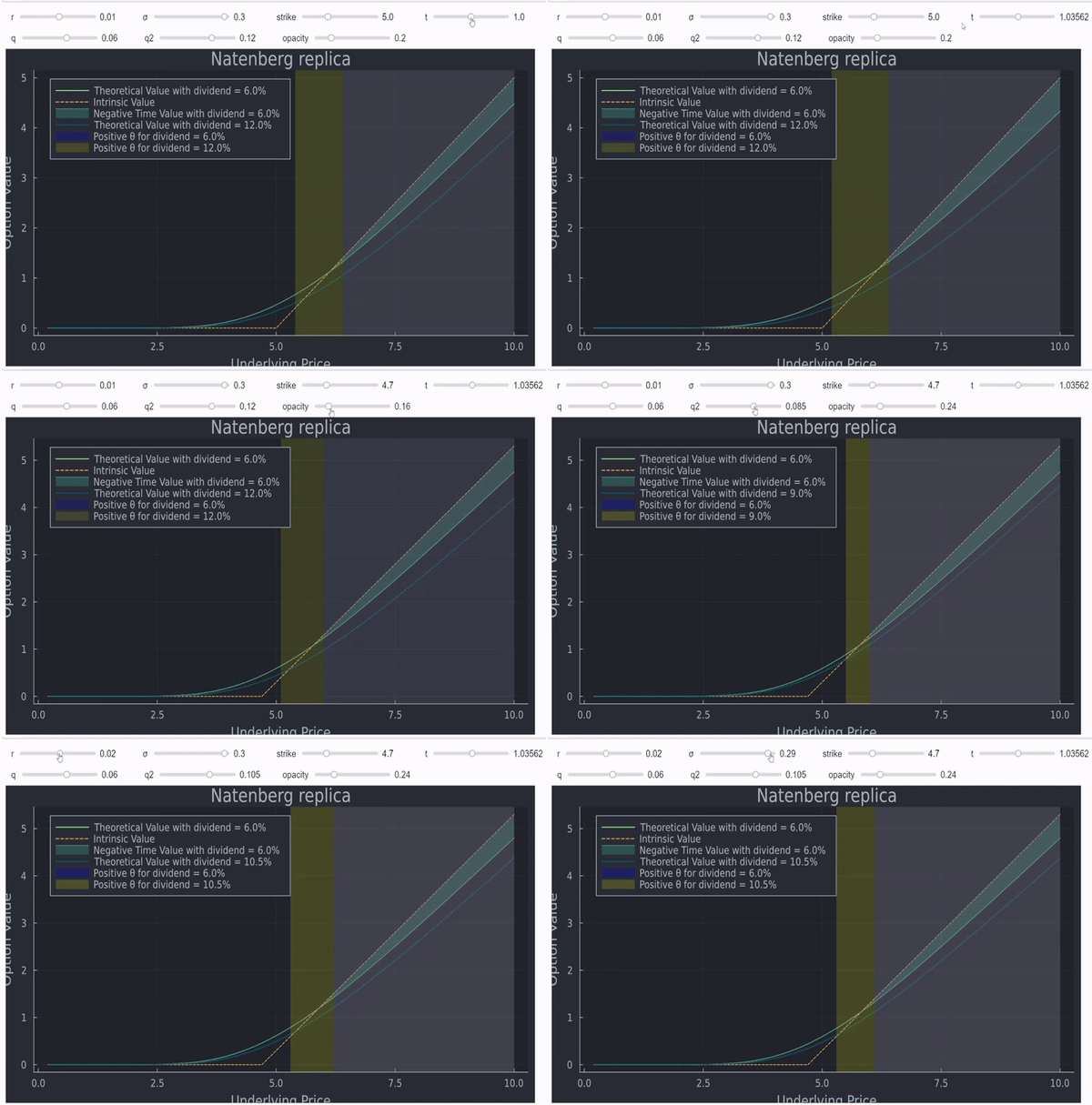
However, with equity options you have another problem. Many stock options are American. As such, your position may be subject to early exercise. here are 2 circumstances that can lead to the value of an European option being lower than intrinsic value

• a) deep ITM puts in presence of positive interest rates r>0
• b ) deep ITM calls in presence of positive dividend yield q>0

which also coincides with the 2 circumstances under which it makes sense for an American option to be exercised early (which can matter for synthetic equity forwards). Some intuition is given here, where the graphic below is taken from.

Any area that is shaded (to the right) will mean early exercise for American options. Insofar, you do not really own a synthetic forward, because if spot moves significantly, one of your legs will be terminated early. On top of that, these options are frequently a lot less liquid compared to the future and as Jan Stuller wrote, you will have two transactions instead of one.

Edit

I highlighted the formula in blue to show that cost of carry is fully integrated into BSM. I mentioned that Black (for pricing option on futures) does not need this cost of carry adjustment because there is no cost or carry for futures. I wrote that cost of carry plays no further role besides determining the fair future (or strike). I added all code and numerical examples. Now, all that is left is to try out a few different values to see that there is indeed no such thing as moneyness or delta adjusted carry. The cost of carry is simply a no arbitrage formula that means no one is made better or worse - hence there is no upfront cost.

Let's look at a numerical example where we do not use the fair strike. As shown above, for ATM spot, the value for a call and put are not identical and the options cost 12.0027 and 11.0371 respectively, hence a total cost of ~0.9656. A shown, the fair forward is $f = s*exp((r-d)*t) \approx 101.005$. Discounting the difference (there is always time value for everything) gives you $(f-k)*e^{-r*t} \approx 0.9656$. That it matches the difference between the call and put is no coincidence, but a simple correction for the unfair (synthetic) forward you enter. This works with any value of interest rates, dividends, IV and whatever else concerns option pricing (as long as you we are talking about European options). Below is the (somewhat messy) code, that creates the DataFrame from the very top. The highligthed lines indicate where K changes (and IV starts to iterate from the beginning).

# define range of volatilities 
σ = 0.1:0.1:1
#compute fair forward
f = s*exp((r-d)*t)
# try a few different strikes (ATM, OTM, ITM)
k,k2,k0 = 102,98,f

# define Black Scholes for the strikes 
call, call2, call0 = BSM.(s,k,t,r,d,σ,1),BSM.(s,k2,t,r,d,σ,1), BSM.(s,k0,t,r,d,σ,1)
put, put2, put0 = BSM.(s,k,t,r,d,σ,-1), BSM.(s,k2,t,r,d,σ,-1), BSM.(s,k0,t,r,d,σ,-1)
call_Black,call_Black2, call_Black0 = Black76.(f,k,t,r,σ,1), Black76.(f,k2,t,r,σ,1), Black76.(f,k0,t,r,σ,-1)
put_Black, put_Black2, put_Black0 = Black76.(f,k,t,r,σ,-1), Black76.(f,k2,t,r,σ,-1), Black76.(f,k0,t,r,σ,-1)

# create result arrays
vols = append!(append!([σ[i] for i in 1:1:length(σ)],[σ[i] for i in 1:1:length(σ)], [σ[i] for i in 1:1:length(σ)]))
c = append!(append!([call0[i][1] for i in 1:1:length(σ)], [call[i][1] for i in 1:1:length(σ)], [call2[i][1] for i in 1:1:length(σ)]))
p = append!(append!([put0[i][1] for i in 1:1:length(σ)], [put[i][1] for i in 1:1:length(σ)],[put2[i][1] for i in 1:1:length(σ)]))
c_black = append!(append!([call_Black0[i][1] for i in 1:1:length(σ)], [call_Black[i][1] for i in 1:1:length(σ)],[call_Black2[i][1] for i in 1:1:length(σ)]))
p_black = append!(append!([put_Black0[i][1] for i in 1:1:length(σ)], [put_Black[i][1] for i in 1:1:length(σ)],[put_Black2[i][1] for i in 1:1:length(σ)]))

# create dataframe 
df = DataFrame("IV" => vols , 
               "C" => c, "P" => p, 
               "C Black" => c_black, "P Black" => p_black,
               "Fwd" => f,
               "Strike"  => append!(append!([k0 for i in 1:1:length(σ)], [k for i in 1:1:length(σ)],[k2 for i in 1:1:length(σ)])),
               "C - P" => [round(c[i][1].-p[i][1],digits =3)  for i in 1:1:length(vols)],
               "(F-K)*e^(-r*t)" => append!(append!([round((f-k0)*exp(-r*t),digits = 3) for i in 1:1:length(σ)], [round((f-k)*exp(-r*t),digits = 3) for i in 1:1:length(σ)],[round((f-k2)*exp(-r*t),digits =3) for i in 1:1:length(σ)]))
)
## put call parity computations for call and put 
df[!, "PCP C"] = round.(df.P .- exp(-r*t).*df.Strike .+ s*exp(-d*t), digits = 4)
df[!, "PCP P"] = round.(df.C .+ exp(-r*t).*df.Strike .- s*exp(-d*t), digits = 4)

# PrettyTables formatting 
hl_1 = Highlighter((data,i,j) -> data[i,1] == 0.100, crayon"bg:dark_gray white bold")
h2 = Highlighter( (data,i,j)->j in (8, 9) && data[i, j] == 2.887,
                         bold       = true,
                         foreground = :blue )
h3 = Highlighter( (data,i,j)->j in (8, 9) && data[i, j] == 0.000,
                         bold       = true,
                         foreground = :green )
PrettyTables.pretty_table(df,  border_crayon = Crayons.crayon"blue", header_crayon = Crayons.crayon"bold green", formatters = ft_printf("%.3f", [1,2,3,4,5,6,7,8,9,10,11]), highlighters = (hl_1, hl_value(-0.956), h2,h3)) 

Julia Ad-on

Unrelated to the question, but the animation is pure Julia code. The sliders (and much more) can be created with Interact. A nice demo (in my opinion, which may be biased because I wrote it) is the very short code below, which plots interactive 3D surfaces of the call value and various greeks in spot and time dimension. As long as Black Scholes is defined (as above just with more Greeks), the actual chart is just 7 lines of code. The quality is reduced here because the allowed GIF size is very small in imgur.

gui = @manipulate for K=K_range, rf=rf_range,d=d_range,σ = 0.01:0.1:1.11,α=0.1:0.1:1, side = 10:1:45,up = 20:2:52;  
    z = [Surface((spot,time)->BSM.(spot,K,time,rf,d,σ)[i], spot, time) for i in 1:1:6]
    title = ["Call Value", "Vega","Delta","Gamma","Theta","Rho"]
    p = [surface(spot,time,z[i], camera=(12,20),α=0.8 ,xlabel="Spot",ylabel="time",title=title[i],legend = :none) for i in 1:1:6]
    plot(p[1],p[2],p[3],p[4],p[5],p[6],layout=(3,3), size =(1000,800))
end
@layout! gui vbox(vbox(hbox(K,rf,d,σ),hbox(α,side,up)), observe(_))

In case anyone is interested in Julia, I did some work a while ago which I partially shared on Econ Stack to showcase why Julia is not slowing you down (unless your code is written in non-performant ways).

Answer 2

I think it's best if we go through the various terms that appear in your question and explain them one-by-one.

Derivative price: intuitively, a derivative price is what it costs to "create it".

Stock forward price: If somebody asks me to sell them an equity forward (i.e. to deliver a stock at some future date), I could "create it" by borrowing some money at an interest rate $r$ (assume continuous compounding) and buying the stock (at price $S_0$) that I am meant to deliver in the future. At the delivery time $t$, I will deliver the stock and will have to pay back the money that I borrowed ($S_0$) times the compounded interest rate: so $S_0e^{rt}$. This is also the price of the stock forward (exactly what it cost to "create it").

If the stock was yielding some dividends between the time I purchased the stock and delivery, I would get to keep those dividends, so you are correct to point out that the dividends would be subtracted from the forward price of the stock (remember, the derivative price is what it costs to make it, so if I get to keep the dividends, it costs me "less", that's why these are subtracted). If we assume continuous compounding of the dividends at rate $y$, then the forward price would be: $S_0e^{rt-yt}$

Stock future price: basically, the difference between a forward and a future is that a stock forward is traded OTC, whilst a future is exchange traded. There will be some subtle pricing differences related to the interest rates in the margining account on the futures exchange. Also, futures tend to be cash-settled. For simplicity, we can assume the same price as a stock forward.

Cost of carry: This is defined as the cost of holding a security or a physical commodity over a period of time. If I were to "create" a forward on oil with a physical delivery, I could borrow money again and buy the required amount of oil, but I'd need to store the oil somewhere: and this would cost money (storage, security). So it would cost more money in general to "create" a physical commodity forward (such as oil, grain, corn, etc.), compared to a stock forward.

Strictly speaking, a security, such as a stock, doesn't have any associated cost of carry. When you say that the future's value converges to the spot value, that's not a cost of carry: it just means that as the future gets closer to maturity, the "time" value of it approaches zero. In other words, the stock future has a negative Theta (sensitivity to remaining time to maturity): but this sensitivity is relatively small, compared to Delta: i.e. sensitivity to the underlying stock value.

Synthetic stock forward: as you rightly point out, the same pay-off as a stock forward can be obtained by being long a call and short a put (with identical strikes) on the same stock. If I am trying to replicate an "at-the-money" forward, the price of the bought call and the price of the sold put should be equal, so it should cost zero.

Price of a Forward contract: In the first paragraph, we discussed that if we agree today that I sell you a (non-dividend paying) stock in the future for the price of $S_0e^{rt}$, it should cost you zero money today to enter into this contract, because we agreed to trade the stock at the future date for a "fair price": exactly what it would cost me to make sure that I can deliver the stock in the future. This is analogous to buying a synthetic forward (a long call and a short put) for net-zero cost.

However, if you wanted to agree to buy the stock at a different price than the fair price (either higher or lower), the cost of the forward contract would be non-zero. Say the stock price today is $S_0$ but you wanted to buy it in the future for less than that: you would need to pay me (today's value) of the difference between the fair value of the stock future price and the specific price you want to buy it for in the future.

This is analogous to the synthetic-forward case where the price of the call is higher than the price of the put: it means that the call is struck in the money, whilst the put is struck out of the money.

Again, there is no real cost of carry here: you paid money upfront for the privilege to have exposure to a better upside in the future. Your main concern is not "the cost of carry" anyway, but the Delta sensitivity to the underlying stock: for each dollar that the underlying stock goes up, you make one dollar, and for each dollar that the underlying stock goes down, you lose one dollar. That's the same for the synthetic forward and the non-synthetic forward.

Interest rates: these generally have small effect on option prices (it's only noticeable on longer-dated options: calls would increase slightly in price, whilst puts would decrease). So it would become slightly more expensive to hold ITM call and be short OTM put. (But this increase in cost should be immaterial for any options with expiry less than 1-year).

Note: however as I show below, the option's sensitivity to rates is a function of the strike price, so if the underlying has a "high" spot value, such as Nasdaq (which has a spot of ~12,000, an unusually high spot compared to stocks), and therefore the strike is also relatively high, the impact of higher rates can be material: see section on Rho below.

Not sure this answers your question, but at least it might help clear up some of the terms.

Zero Cost Synthetic Forward:

We want the long call and the short put to cost the same, for a given expiry $T$, today's underlying price $S_0$, interest rates $r$, and implied volatility $\sigma$: in other words, we want to solve for a strike $K$ in the following equation (within the B-S framework):

$$P(t_0, S_0, T, r, \sigma, K)=C(t_0, S_0, T, r, \sigma, K)$$

In other words:

$$e^{-rT}KN(-d_2)-S_0N(-d_1)=S_0N(d_1)-e^{-rT}KN(d_2)$$

Bringing all terms to the RHS:

$$0=S_0\left(N(d_1)+N(-d_1)\right)-e^{-rT}K\left(N(d_2)+N(-d_2)\right) \{eq. 1\}$$

Where:

$$d_1=\frac{\ln\left(\frac{S_0}{K}\right)+rT+0.5\sigma^2T}{\sigma\sqrt{T}}, d_2=\frac{\ln\left(\frac{S_0}{K}\right)+rT-0.5\sigma^2T}{\sigma\sqrt{T}}$$

Choosing $K=e^{rt}S_0$, we get (using the fact that $ln\left(\frac{S_0}{S_0e^rt}\right)=-e^{rt})$:

$$N(d_1)=N(0.5\sigma\sqrt{T})\approx0.5; N(-d_1)=N(-0.5\sigma\sqrt{T})\approx0.5$$

and also:

$$N(d_2)=N(-0.5\sigma\sqrt{T})\approx0.5; N(-d_2)=N(0.5\sigma\sqrt{T})\approx0.5$$

Going back to eq. 1:

$$0=^{?}S_0(0.5+0.5)-e^{-rT}e^{rt}S_0\left(0.5+0.5\right)=S_0-S_0=0$$

As required.

So we have shown that a long call and a short put, struck ATM, should cost very close to net-zero.

(btw, even if we don't use the approximation $N(-0.5\sigma\sqrt{T})\approx0.5$, by symmetry, we have that $N(-0.5\sigma\sqrt{T})+N(0.5\sigma\sqrt{T})=1$ in any case).

Broker Fees:

If there is an initial broker fee to enter into a long Nasdaq future contract, this should not be confused with a cost of carry.

Buying and selling options at a broker will attract a bid-offer spread. This will mean that in practice, a long ATM call and a short ATM put will require an initial investment (even though the mid-prices should make the strategy cost zero): you will have to cross the spread twice (hitting broker's offer on the call and hitting broker's bid on the put).

Whether the initial cost of being long the future is higher than doing a synthetic long via options will depend on individual broker fees. But my guess would be that the future should be cheaper, because you only cross the bid-offer once, whereas in options, you cross it twice + options are probably less liquid than the futures (meaning a larger bid-offer).

Rho - price sensitivity to rates:

As discussed above, the ATM futures price, $S_t$, is simply:

$$S_t=S_0e^{rt-yt}$$.

The sensitivity to interest rates, $\rho$, would be (the formula below gives sensitivity to 1% change in rates, that's why we have $\frac{1}{100}$ in the formula):

$$\rho=\frac{1}{100}\frac{\partial S_t}{\partial r}=\frac{1}{100}tS_0e^{rt-yt}$$

Assuming 3m expiry (therefore $t=0.25$), the future's sensitivity to 1% change in interest rates would therefore be $\frac{1}{400}$ of it's today's ATM value.

Concrete example:

Suppose today's price of Nasdaq is 12,000, interest rates are at 1%, and dividends are at zero (for simplicity). Then the ATM price of a futures contract expiring in 3 months would be: $$12,000e^{0.01*0.25}=12,030$$

Suppose rates go to 5% (current upper band of Fed Funds target rate); using the sensitivity formula, we get:

$$\rho=\frac{4}{400}12,030=120.3$$

So the futures ATM strike would have gone up by ~120 USD, i.e. from ~12,030 USD to ~12,150 USD.

What about the price of options?

We denote the option's sensitivity to rates also $\rho$. For calls, this is:

$$\rho(Call)=\frac{1}{100}KTe^{-Tr}N(d_2)$$

Above, we argued that for an ATM option, $N(d_2)\approx0.5$, and filling in all other variables, we get:

$$\rho(Call)=\frac{1}{100}12,030*0.25e^{-0.25*0.01}0.5\approx15$$

So for every increase in interest rates by 1%, the ATM call price would increase by roughly 15 USD (so an increase from 1% to 5% would mean a 60 USD increase).

Note that the Rho value for the put is the opposite of the Rho for the call:

$$\rho(Put)=-\frac{1}{100}KTe^{-Tr}N(d_2)$$

So for every 1% increase in rates, the put price would decrease by roughly 15 USD.

Delta sensi: lastly, let's ask the question of whether I can "save" on the "cost-of-carry" if, instead of doing a synthetic forward struck at 12,150 USD, I want to strike it at exactly today's value of Nasdaq spot (assume that's still 12,000 USD).

Earlier on above, we argued that for ATM calls, $N(d1)\approx0.5$. In fact, $N(d1)$ is the call-option delta.

For puts, the delta is $-N(-d1)$, so for ATM puts, the delta is the opposite of the call delta, i.e. -0.5.

If we want an easy "guestimate" of how much more expensive it will be to set up a synthetic forward struck at 12,000 instead of 12,150, that's easy using the delta.

For the call:

$$\delta(150)\approx0.5*150=75$$

For the put:

$$\delta(150)\approx-0.5*150=-75$$

So the call would get more expensive by 75 USD, if we move the strike from 12,150 to 12,000, whilst the put would get 75 USD cheaper.

Since for the synthetic long forward, we are long the call and short the put, the strategy would get more expensive by 150 USD: i.e. the exact amount I would "save" on the future's "cost-of-carry".

Which ever way we look at it, there is no free lunch.

Rule of thumb: if two strategies offer the same pay-off, they will always cost the same amount to set up (with broker fees & bid-offer spreads, there might be some differences, but in terms of "pricing at mid", the cost must be identical, otherwise there would be arbitrage).

Answer 3

Interest rates have an effect on options in two ways:

1. the forward: the higher the interest rates, the higher the forward. Thus with a higher forward, calls become more expensive and put the opposite.
2. The present value of the premium: The price of the option = PV(E[Payoff]). So with higer interest rates, premiums prices will go down, both for calls and puts, regarding this effect.

Now how do we link these effects to carry?

The first one will be indeed proportional to delta, as you expect the spot to climb a little bit every day until it reaches the forward. Every day spot does not go up, the call will depreciate a little bit due to this effect, and the put will appreciate. If it is a deep ITM option it will have a large effect, as the option will be comparable to a forward outright.

The second effect will also depend if the option is ITM or OTM but in another way: if the option is ITM it will have more premium than its counterpart. The carry that this generates is simply E[premium at $t+1$] - premium at $t_0$, which is basically removing 1 day of discounting from the E[payoff].